NumPy 난수 생성 (Random 모듈)¶

NumPy 패키지의 random 모듈 (numpy.random)에 대해 소개합니다.

random 모듈의 다양한 함수를 사용해서 특정 범위, 개수, 형태를 갖는 난수 생성에 활용할 수 있습니다.

■ Table of Contents

random.rand()
random.randint()
random.randn()
random.standard_normal()
random.normal()
random.random_sample()
random.choice()
random.seed()

random.rand()¶

random.rand() 함수는 주어진 형태의 난수 어레이를 생성합니다.

예제1 - 기본 사용¶

import numpy as np

a = np.random.rand(5)
print(a)

b = np.random.rand(2, 3)
print(b)

[0.41626628 0.40269923 0.80574938 0.67014962 0.47630372]

[[0.83739956 0.62462355 0.66043459]
 [0.96358531 0.23121274 0.68940178]]

만들어진 난수 어레이는 주어진 값에 의해 결정되며, [0, 1) 범위에서 균일한 분포를 갖습니다.

예제2 - Matplotlib 시각화¶

import numpy as np
import matplotlib.pyplot as plt

np.random.seed(0)

plt.style.use('default')
plt.rcParams['figure.figsize'] = (6, 3)
plt.rcParams['font.size'] = 12

a = np.random.rand(1000)
b = np.random.rand(10000)
c = np.random.rand(100000)

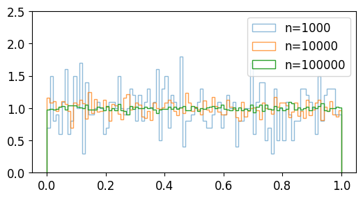
plt.hist(a, bins=100, density=True, alpha=0.5, histtype='step', label='n=1000')
plt.hist(b, bins=100, density=True, alpha=0.75, histtype='step', label='n=10000')
plt.hist(c, bins=100, density=True, alpha=1.0, histtype='step', label='n=100000')

plt.ylim(0, 2.5)
plt.legend()
plt.show()

NumPy와 Matplotlib을 이용해서 난수의 분포를 확인해보면,

샘플의 개수가 1000, 10000, 100000개로 증가할수록 더욱 균일한 분포를 보임을 알 수 있습니다.

NumPy 난수 생성 (Random 모듈) - random.rand()¶

random.randint()¶

random.randint() 함수는 [최소값, 최대값)의 범위에서 임의의 정수를 만듭니다.

예제1 - 기본 사용¶

import numpy as np

a = np.random.randint(2, size=5)
print(a)

b = np.random.randint(2, 4, size=5)
print(b)

c = np.random.randint(1, 5, size=(2, 3))
print(c)

[0 0 0 0 0]

[3 3 2 2 3]

[[3 2 4]
 [2 2 2]]

np.random.randint(2, size=5)는 [0, 2) 범위에서 다섯개의 임의의 정수를 생성합니다.

np.random.randint(2, 4, size=5)는 [2, 4) 범위에서 다섯개의 임의의 정수를 생성합니다.

np.random.randint(1, 5, size=(2, 3))는 [1, 5) 범위에서 (2, 3) 형태의 어레이를 생성합니다.

예제2 - Matplotlib 시각화¶

import numpy as np
import matplotlib.pyplot as plt

plt.style.use('default')
plt.rcParams['figure.figsize'] = (6, 3)
plt.rcParams['font.size'] = 12

a = np.random.randint(0, 10, 1000)
b = np.random.randint(10, 20, 1000)
c = np.random.randint(0, 20, 1000)

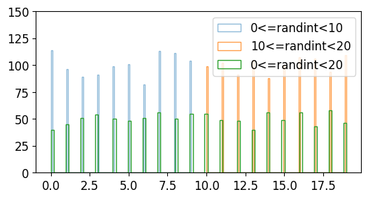
plt.hist(a, bins=100, density=False, alpha=0.5, histtype='step', label='0<=randint<10')
plt.hist(b, bins=100, density=False, alpha=0.75, histtype='step', label='10<=randint<20')
plt.hist(c, bins=100, density=False, alpha=1.0, histtype='step', label='0<=randint<20')

plt.ylim(0, 150)
plt.legend()
plt.show()

a는 [0, 10) 범위의 임의의 정수 1000개,

b는 [10, 20) 범위의 임의의 정수 1000개,

c는 [0, 20) 범위의 임의의 정수 1000개입니다.

분포를 확인해보면 아래와 같습니다.

NumPy 난수 생성 (Random 모듈) - random.randint()¶

random.randn()¶

random.randn() 함수는 표준정규분포 (Standard normal distribution)로부터 샘플링된 난수를 반환합니다.

예제1 - 기본 사용¶

import numpy as np

a = np.random.randn(5)
print(a)

b = np.random.randn(2, 3)
print(b)

sigma, mu = 1.5, 2.0

c = sigma * np.random.randn(5) + mu
print(c)

[ 0.06704336 -0.48813686  0.4275107  -0.9015714  -1.30597604]

[[ 0.87354043  0.03783873  0.77153503]
 [-0.35765934  2.11477207  1.28474164]]

[0.47894537 1.2894864  2.51428183 1.55888021 0.08079876]

표준정규분포 N(1, 0)이 아닌, 평균 \({\mu}\), 표준편차 \({\sigma}\) 를 갖는 정규분포 N(\({\mu}\), \({\sigma}\)²)의 난수를 생성하기 위해서는

\({\sigma}\) * np.random.randn(…) + \({\mu}\) 와 같은 형태로 사용할 수 있습니다.

예제2 - Matplotlib 시각화¶

import numpy as np
import matplotlib.pyplot as plt

plt.style.use('default')
plt.rcParams['figure.figsize'] = (6, 3)
plt.rcParams['font.size'] = 12

a = np.random.randn(100000)
b = 2 * np.random.randn(100000) - 1
c = 4 * np.random.randn(100000) + 2

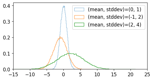
plt.hist(a, bins=100, density=True, alpha=0.5, histtype='step', label='(mean, stddev)=(0, 1)')
plt.hist(b, bins=100, density=True, alpha=0.75, histtype='step', label='(mean, stddev)=(-1, 2)')
plt.hist(c, bins=100, density=True, alpha=1.0, histtype='step', label='(mean, stddev)=(2, 4)')

plt.xlim(-15, 25)
plt.legend()
plt.show()

a는 평균과 표준편차가 각각 0, 1인 정규분포의 난수 100000개,

b는 평균과 표준편차가 각각 -1, 2인 정규분포의 난수 100000개,

c는 평균과 표준편차가 각각 2, 4인 정규분포의 난수 100000개입니다.

분포를 확인해보면 아래와 같습니다.

NumPy 난수 생성 (Random 모듈) - random.randn()¶

random.standard_normal()¶

random.standard_normal() 함수는 표준정규분포 (Standard normal distribution)로부터 샘플링된 난수를 반환합니다.

standard_normal() 함수는 randn() 함수와 비슷하지만, 튜플을 인자로 받는다는 점에서 차이가 있습니다.

예제1 - 기본 사용¶

import numpy as np

d = np.random.standard_normal(3)
print(d)

e = np.random.standard_normal((2, 3))
print(e)

[ 0.72496842 -1.94269564 -0.39983457]

[[-0.36962525  0.61226929  1.91266759]
 [ 0.2095275  -0.66655062  0.74094405]]

예제2 - Matplotlib 시각화¶

import numpy as np
import matplotlib.pyplot as plt

plt.style.use('default')
plt.rcParams['figure.figsize'] = (6, 3)
plt.rcParams['font.size'] = 12

a = np.random.standard_normal(1000)
b = np.random.standard_normal(10000)
c = np.random.standard_normal(100000)

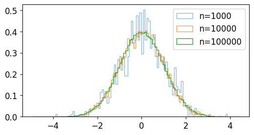
plt.hist(a, bins=100, density=True, alpha=0.5, histtype='step', label='n=1000')
plt.hist(b, bins=100, density=True, alpha=0.75, histtype='step', label='n=10000')
plt.hist(c, bins=100, density=True, alpha=1.0, histtype='step', label='n=100000')

plt.legend()
plt.show()

a는 표준정규분포를 갖는 난수 1000개,

b는 표준정규분포를 갖는 난수 10000개,

c는 표준정규분포를 갖는 난수 100000개입니다.

분포를 확인해보면 아래와 같습니다.

NumPy 난수 생성 (Random 모듈) - random.standard_normal()¶

random.normal()¶

random.normal() 함수는 정규 분포 (Normal distribution)로부터 샘플링된 난수를 반환합니다.

예제1 - 기본 사용¶

import numpy as np

a = np.random.normal(0, 1, 2)
print(a)

b = np.random.normal(1.5, 1.5, 4)
print(b)

c = np.random.normal(3.0, 2.0, (2, 3))
print(c)

[-0.66144234  2.52980783]
[2.96297363 1.71391993 1.61165712 3.57817189]
[[3.28846179 5.14251661 4.31800249]
[4.79395804 1.59956438 4.46791867]]

어레이 a는 정규 분포 \(N(0, 1)\)로부터 얻은 임의의 숫자 2개,

어레이 b는 정규 분포 \(N(1.5, 1.5^2)\)로부터 얻은 임의의 숫자 4개,

어레이 c는 정규 분포 \(N(3.0, 2.0^2)\)로부터 얻은 (2, 3) 형태의 임의의 숫자 어레이입니다.

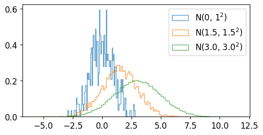
예제2 - Matplotlib 시각화¶

import numpy as np
import matplotlib.pyplot as plt

plt.style.use('default')
plt.rcParams['figure.figsize'] = (6, 3)
plt.rcParams['font.size'] = 12

a = np.random.normal(0, 1, 500)
b = np.random.normal(1.5, 1.5, 5000)
c = np.random.normal(3.0, 2.0, 50000)

plt.hist(a, bins=100, density=True, alpha=0.75, histtype='step', label=r'N(0, $1^2$)')
plt.hist(b, bins=100, density=True, alpha=0.75, histtype='step', label=r'N(1.5, $1.5^2$)')
plt.hist(c, bins=100, density=True, alpha=0.75, histtype='step', label=r'N(3.0, $3.0^2$)')

plt.legend()
plt.show()

a는 정규 분포를 갖는 난수 500개,

b는 정규 분포를 갖는 난수 5000개,

c는 정규 분포를 갖는 난수 50000개입니다.

분포를 확인해보면 아래와 같습니다.

NumPy 난수 생성 (Random 모듈) - random.normal()¶

random.random_sample()¶

random.random_sample() 함수는 [0.0, 1.0) 범위에서 샘플링된 임의의 실수를 반환합니다.

예제1 - 기본 사용¶

import numpy as np

a = np.random.random_sample()
print(a)

b = np.random.random_sample((5, 2))
print(b)

c = 5 * np.random.random_sample((3, 2)) - 3
print(c)

0.9662064052518934

[[0.21827699 0.39935976]
 [0.4444503  0.53683571]
 [0.63821048 0.89894424]
 [0.07794204 0.80244891]
 [0.36607828 0.15745157]]

[[ 1.17525258  0.58536383]
 [ 1.44294647 -2.39544082]
  [-0.48931127  1.84401433]]

주어진 범위와 형태를 갖는 난수의 어레이를 반환합니다.

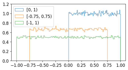
예제2 - Matplotlib 시각화¶

import numpy as np
import matplotlib.pyplot as plt

plt.style.use('default')
plt.rcParams['figure.figsize'] = (6, 3)
plt.rcParams['font.size'] = 12

a = np.random.random_sample(100000)
b = 1.5 * np.random.random_sample(100000) - 0.75
c = 2 * np.random.random_sample(100000) - 1

plt.hist(a, bins=100, density=True, alpha=0.75, histtype='step', label='[0, 1)')
plt.hist(b, bins=100, density=True, alpha=0.75, histtype='step', label='[-0.75, 0.75)')
plt.hist(c, bins=100, density=True, alpha=0.75, histtype='step', label='[-1, 1)')

plt.ylim(0.0, 1.2)
plt.legend()
plt.show()

[0.0, 1.0) 범위가 아닌 [a, b) 범위의 난수를 생성하려면,

(b-a) * random_sample() + a와 같이 생성하면 됩니다.

분포는 아래와 같습니다.

NumPy 난수 생성 (Random 모듈) - random.random_sample()¶

random.choice()¶

random.choice() 함수는 주어진 1차원 어레이로부터 임의의 샘플을 생성합니다.

예제1 - 기본 사용¶

import numpy as np

a = np.random.choice(5, 3)
print(a)

b = np.random.choice(10, (2, 3))
print(b)

[4 0 2]
[[0 2 1]
 [4 7 2]]

어레이 a는 np.arange(5)에서 3개의 샘플을 뽑은 1차원 어레이입니다.

어레이 b는 np.arange(10)에서 샘플을 뽑은 (2, 3) 형태의 어레이입니다.

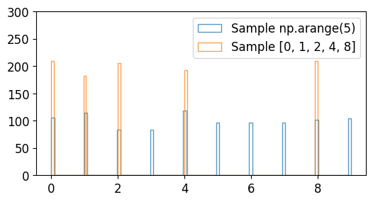
예제2 - Matplotlib 시각화¶

import numpy as np
import matplotlib.pyplot as plt

plt.style.use('default')
plt.rcParams['figure.figsize'] = (6, 3)
plt.rcParams['font.size'] = 12

a = np.random.choice(10, 1000)
b = np.random.choice([0, 1, 2, 4, 8], 1000)

plt.hist(a, bins=100, density=False, alpha=0.75, histtype='step', label='Sample np.arange(5)')
plt.hist(b, bins=100, density=False, alpha=0.75, histtype='step', label='Sample [0, 1, 2, 4, 8]')

plt.ylim(0, 300)
plt.legend()
plt.show()

a는 np.arange(10)에서 임의로 뽑은 1000개의 샘플

b는 [0, 1, 2, 4, 8]에서 임의로 뽑은 1000개의 샘플입니다.

분포는 아래와 같습니다.

NumPy 난수 생성 (Random 모듈) - random.choice()¶

random.seed()¶

random.seed() 함수는 난수 생성에 필요한 시드를 설정합니다.

예제¶

import numpy as np

np.random.seed(0)

print(np.random.rand(2, 3))

[[0.5488135  0.71518937 0.60276338]
 [0.54488318 0.4236548  0.64589411]]

(2, 3) 형태의 2차원 난수 어레이가 생성되었습니다.

코드를 실행할 때마다 동일한 난수가 생성됩니다.

이전글 : 어레이 쪼개기

다음글 : NumPy 다양한 함수들

NumPy 난수 생성 (Random 모듈)¶

random.rand()¶

예제1 - 기본 사용¶

예제2 - Matplotlib 시각화¶

random.randint()¶

예제1 - 기본 사용¶

예제2 - Matplotlib 시각화¶

random.randn()¶

예제1 - 기본 사용¶

예제2 - Matplotlib 시각화¶

random.standard_normal()¶

예제1 - 기본 사용¶

예제2 - Matplotlib 시각화¶

random.normal()¶

예제1 - 기본 사용¶

예제2 - Matplotlib 시각화¶

random.random_sample()¶

예제1 - 기본 사용¶

예제2 - Matplotlib 시각화¶

random.choice()¶

예제1 - 기본 사용¶

예제2 - Matplotlib 시각화¶

random.seed()¶

예제¶

관련 페이지¶

이전글/다음글