[확률과 통계] 파이썬으로 정규 분포 그리기
■ Table of Contents
1. 정규 분포란
정규 분포 (Normal distribution)는 통계학에서 연속 확률 분포의 한 종류로서 데이터의 분포를 근사하는데 가장 흔하게 사용됩니다.
정규 분포는 가우스 분포 (Gaussian distribution)라고도 합니다.
정규 분포의 모양은 2개의 매개 변수인 평균 \(\mu\)과 표준편차 \(\sigma\)에 의해 결정되며, 이 때의 분포를 \(N(\mu, \sigma^2)\)으로 나타냅니다.
정규 분포 \(N(\mu, \sigma^2)\)를 갖는 확률 변수 \(x\)는 기대값, 최빈값, 중앙값이 모두 \(\mu\)이며, 분산은 \(\sigma^2\)로 주어집니다.
정규 분포 \(N(\mu, \sigma^2)\)를 갖는 확률 변수 \(x\)에 대한 확률 밀도 함수 (Probability Density Function)는 아래와 같이 주어집니다.
또한 정규 분포 \(N(\mu, \sigma^2)\)의 확률 밀도 함수에 대한 누적 분포 함수 (Cumulative Distribution Function)는 아래와 같이 주어집니다.
2. 정규 분포 그리기
import numpy as np
import matplotlib.pyplot as plt
from scipy.special import erf

np.random.seed(0)

plt.style.use('default')
plt.rcParams['figure.figsize'] = (6, 3)
plt.rcParams['font.size'] = 12
plt.rcParams['lines.linewidth'] = 5

mu = 0.0
sigma = 1.0

x = np.linspace(-8, 8, 1000)
y = (1 / np.sqrt(2 * np.pi * sigma**2)) * np.exp(-(x-mu)**2 / (2 * sigma**2))
y_cum = 0.5 * (1 + erf((x - mu)/(np.sqrt(2 * sigma**2))))

plt.plot(x, y, alpha=0.7, label='PDF of N(0, 1)')
plt.plot(x, y_cum, alpha=0.7, label='CDF of N(0, 1)')
plt.xlabel('x')
plt.ylabel('f(x)')
plt.legend(loc='upper left')
plt.show()
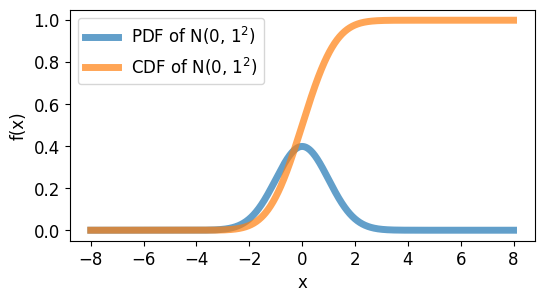
이 예제 코드는 파이썬, NumPy, Matplotlib, 그리고 SciPy 라이브러리를 사용해서
평균 (mu) 0.0, 표준편차 (sigma) 1.0을 갖는 정규 분포의 확률 밀도 함수와 누적 분포 함수를 나타냅니다.
결과는 아래와 같습니다.
파이썬으로 정규 분포 그리기 - 정규 분포 그리기
3. 평균과 표준편차
import numpy as np
import matplotlib.pyplot as plt

np.random.seed(0)

plt.style.use('default')
plt.rcParams['figure.figsize'] = (6, 3)
plt.rcParams['font.size'] = 12
plt.rcParams['lines.linewidth'] = 5

mu1, sigma1 = 0.0, 1.0
mu2, sigma2 = 1.5, 1.5
mu3, sigma3 = 3.0, 2.0

x = np.linspace(-8, 8, 1000)
y1 = (1 / np.sqrt(2 * np.pi * sigma1**2)) * np.exp(-(x-mu1)**2 / (2 * sigma1**2))
y2 = (1 / np.sqrt(2 * np.pi * sigma2**2)) * np.exp(-(x-mu2)**2 / (2 * sigma2**2))
y3 = (1 / np.sqrt(2 * np.pi * sigma3**2)) * np.exp(-(x-mu3)**2 / (2 * sigma3**2))

plt.plot(x, y1, alpha=0.7, label=r'PDF of N(0, $1^2$)')
plt.plot(x, y2, alpha=0.7, label=r'PDF of N(1.5, $1.5^2$)')
plt.plot(x, y3, alpha=0.7, label=r'PDF of N(3.0, $2.0^2$)')
plt.xlabel('x')
plt.ylabel('f(x)')
plt.legend(bbox_to_anchor=(1.0, -0.2))
plt.show()
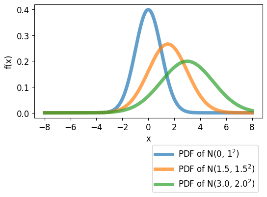
이번에는 각기 다른 평균과 표준편차를 갖는 확률 밀도 함수를 나타냈습니다.
각각 정규 분포 \(N(0, 1^2)\), \(N(1.5, 1.5^2)\), \(N(3.0, 2.0^2)\)를 갖는 확률 밀도 함수는 아래 그림과 같습니다.
이 중에서 평균 0, 표준편차 1을 갖는 정규 분포 \(N(0, 1^2)\)를 표준 정규 분포 (Standard Normal Distribution)이라고 합니다.
파이썬으로 정규 분포 그리기 - 평균과 표준편차
4. np.random.normal()
NumPy random 모듈의 random.normal() 함수는 정규 분포로부터 얻은 임의의 샘플을 반환합니다.
import numpy as np
import matplotlib.pyplot as plt

np.random.seed(0)

plt.style.use('default')
plt.rcParams['figure.figsize'] = (6, 3)
plt.rcParams['font.size'] = 12
plt.rcParams['lines.linewidth'] = 5

mu1, sigma1 = 0.0, 1.0
mu2, sigma2 = 1.5, 1.5
mu3, sigma3 = 3.0, 2.0

x = np.linspace(-8, 8, 1000)
y1 = (1 / np.sqrt(2 * np.pi * sigma1**2)) * np.exp(-(x-mu1)**2 / (2 * sigma1**2))
y2 = (1 / np.sqrt(2 * np.pi * sigma2**2)) * np.exp(-(x-mu2)**2 / (2 * sigma2**2))
y3 = (1 / np.sqrt(2 * np.pi * sigma3**2)) * np.exp(-(x-mu3)**2 / (2 * sigma3**2))

y4 = np.random.normal(mu1, sigma1, 50000)
y5 = np.random.normal(mu2, sigma2, 50000)
y6 = np.random.normal(mu3, sigma3, 50000)

plt.plot(x, y1, alpha=0.7, label=r'PDF of N(0, $1^2$)')
plt.plot(x, y2, alpha=0.7, label=r'PDF of N(1.5, $1.5^2$)')
plt.plot(x, y3, alpha=0.7, label=r'PDF of N(3.0, $2.0^2$)')

plt.hist(y4, bins=1000, density=True, histtype='stepfilled', label=r'random.normal(0, $1^2$)', color='C0')
plt.hist(y5, bins=1000, density=True, histtype='stepfilled', label=r'random.normal(1.5, $1.5^2$)', color='C1')
plt.hist(y6, bins=1000, density=True, histtype='stepfilled', label=r'random.normal(3.0, $2.0^2$)', color='C2')

plt.xlabel('x')
plt.ylabel('f(x)')
plt.xlim(-8.5, 8.5)
plt.legend(ncol=2, bbox_to_anchor=(1.0, -0.2))
plt.show()
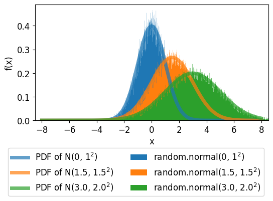
이번에는 정규 분포의 확률 밀도 함수와 함께 random.normal() 함수로부터 얻은 난수를 히스토그램으로 나타냈습니다.
random.normal() 함수의 첫번째 인자로 분포의 평균, 두번째 인자로 분포의 표준편차,
그리고 세번째 인자로 생성할 난수의 개수를 입력합니다.
matplotlib.pyplot 모듈의 hist() 함수는 주어진 숫자 어레이의 분포를 히스토그램으로 나타내며,
density=True로 설정하면 분포를 밀도로서 표현합니다.
(자세한 내용은 Matplotlib 히스토그램 그리기 페이지를 참고하세요.)
아래 그림과 같이 각각의 정규 분포로부터 임의로 얻은 50000개의 난수가 이론적인 정규 분포의 확률 밀도 함수와
잘 일치함을 확인할 수 있으며, 생성한 난수의 개수가 커질 수록 더 잘 일치하는 결과를 확인할 수 있습니다.
파이썬으로 정규 분포 그리기 - np.random.normal()