Contents
- TensorFlow - 구글 머신러닝 플랫폼
- 1. 텐서 기초 살펴보기
- 2. 간단한 신경망 만들기
- 3. 손실 함수 살펴보기
- 4. 옵티마이저 사용하기
- 5. AND 로직 연산 학습하기
- 6. 뉴런층의 속성 확인하기
- 7. 뉴런층의 출력 확인하기
- 8. MNIST 손글씨 이미지 분류하기
- 9. Fashion MNIST 이미지 분류하기
- 10. 합성곱 신경망 사용하기
- 11. 말과 사람 이미지 분류하기
- 12. 고양이와 개 이미지 분류하기
- 13. 이미지 어그멘테이션의 효과
- 14. 전이 학습 활용하기
- 15. 다중 클래스 분류 문제
- 16. 시냅스 가중치 얻기
- 17. 시냅스 가중치 적용하기
- 18. 모델 시각화하기
- 19. 훈련 과정 시각화하기
- 20. 모델 저장하고 복원하기
- 21. 시계열 데이터 예측하기
- 22. 자연어 처리하기 1
- 23. 자연어 처리하기 2
- 24. 자연어 처리하기 3
- 25. Reference
- tf.cast
- tf.constant
- tf.keras.activations.exponential
- tf.keras.activations.linear
- tf.keras.activations.relu
- tf.keras.activations.sigmoid
- tf.keras.activations.softmax
- tf.keras.activations.tanh
- tf.keras.datasets
- tf.keras.layers.Conv2D
- tf.keras.layers.Dense
- tf.keras.layers.Flatten
- tf.keras.layers.GlobalAveragePooling2D
- tf.keras.layers.InputLayer
- tf.keras.layers.ZeroPadding2D
- tf.keras.metrics.Accuracy
- tf.keras.metrics.BinaryAccuracy
- tf.keras.Sequential
- tf.linspace
- tf.ones
- tf.random.normal
- tf.range
- tf.rank
- tf.TensorShape
- tf.zeros
Tutorials
- Python Tutorial
- NumPy Tutorial
- Matplotlib Tutorial
- PyQt5 Tutorial
- BeautifulSoup Tutorial
- xlrd/xlwt Tutorial
- Pillow Tutorial
- Googletrans Tutorial
- PyWin32 Tutorial
- PyAutoGUI Tutorial
- Pyperclip Tutorial
- TensorFlow Tutorial
- Tips and Examples
11. 말과 사람 이미지 분류하기
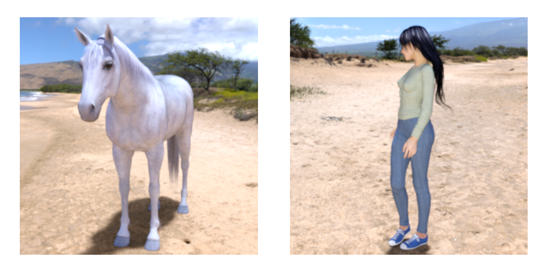
이제 MNIST와 Fashion MNIST보다 더 현실적인 분류 문제인 “말과 사람 이미지 분류하기” 문제를 다룹니다.
순서는 아래와 같습니다.
데이터셋 준비하기
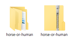
우선 아래의 주소에 접속해서 말과 사람 사진 데이터셋 파일을 다운로드하고, 압축을 풀어줍니다.
URL: https://storage.googleapis.com/laurencemoroney-blog.appspot.com/horse-or-human.zip
지정한 경로에 아래와 같은 폴더가 생성되었다면 준비가 된 것입니다.
데이터셋 살펴보기
경로와 파일명
import os

# horses/humans 데이터셋 경로 지정
train_horse_dir = './tmp/horse-or-human/horses'
train_human_dir = './tmp/horse-or-human/humans'

# horses 파일 이름 리스트
train_horse_names = os.listdir(train_horse_dir)
print(train_horse_names[:10])

# humans 파일 이름 리스트
train_human_names = os.listdir(train_human_dir)
print(train_human_names[:10])

# horses/humans 총 이미지 파일 개수
print('total training horse images:', len(os.listdir(train_horse_dir)))
print('total training human images:', len(os.listdir(train_human_dir)))
['horse01-0.png', 'horse01-1.png', 'horse01-2.png', 'horse01-3.png', 'horse01-4.png', 'horse01-5.png', 'horse01-6.png', 'horse01-7.png', 'horse01-8.png', 'horse01-9.png']
['human01-00.png', 'human01-01.png', 'human01-02.png', 'human01-03.png', 'human01-04.png', 'human01-05.png', 'human01-06.png', 'human01-07.png', 'human01-08.png', 'human01-09.png']
total training horse images: 500
total training human images: 527
말/사람 이미지 데이터셋이 포함된 경로를 각각 train_horse_dir, train_human_dir에 지정합니다.
os.listdir()을 이용해서 경로에 포함된 파일 이름을 리스트 형태로 불러올 수 있습니다.
이 리스트의 길이를 각각 확인해보면 말 이미지가 500개, 사람 이미지가 527개 있음을 알 수 있습니다.
이미지 확인하기
import matplotlib.pyplot as plt
import matplotlib.image as mpimg

nrows = 4
ncols = 4

pic_index = 0

fig = plt.gcf()
fig.set_size_inches(ncols * 4, nrows * 4)

pic_index += 8
next_horse_pix = [os.path.join(train_horse_dir, fname) for fname in train_horse_names[pic_index-8:pic_index]]
next_human_pix = [os.path.join(train_human_dir, fname) for fname in train_human_names[pic_index-8:pic_index]]

for i, img_path in enumerate(next_horse_pix+next_human_pix):
  sp = plt.subplot(nrows, ncols, i + 1)
  sp.axis('Off')

  img = mpimg.imread(img_path)
  plt.imshow(img)

plt.show()
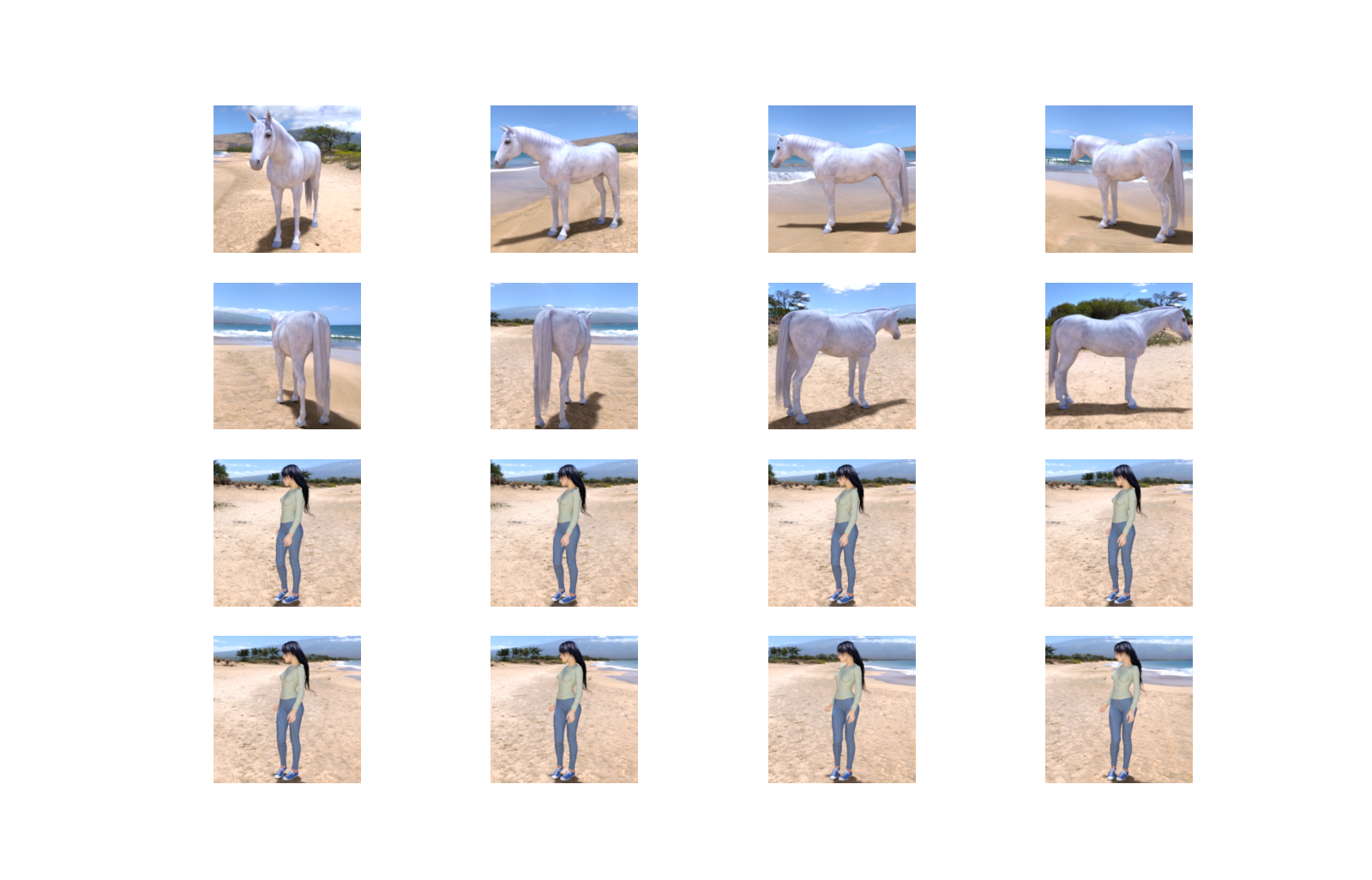
Matplotlib을 이용해서 말과 사람의 이미지를 각각 8개씩 띄워보겠습니다.
결과는 아래와 같습니다.
모델 구성하기
이제 이미지 분류와 훈련을 위한 합성곱 신경망 (Convolutional Neural Network)을 구성합니다.
import tensorflow as tf

model = tf.keras.models.Sequential([
    # The first convolution
    tf.keras.layers.Conv2D(16, (3, 3), activation='relu', input_shape=(300, 300, 3)),
    tf.keras.layers.MaxPool2D(2, 2),
    # The second convolution
    tf.keras.layers.Conv2D(32, (3, 3), activation='relu'),
    tf.keras.layers.MaxPool2D(2, 2),
    # The third convolution
    tf.keras.layers.Conv2D(64, (3, 3), activation='relu'),
    tf.keras.layers.MaxPool2D(2, 2),
    # The fourth convolution
    tf.keras.layers.Conv2D(64, (3, 3), activation='relu'),
    tf.keras.layers.MaxPool2D(2, 2),
    # The fifth convolution
    tf.keras.layers.Conv2D(64, (3, 3), activation='relu'),
    tf.keras.layers.MaxPool2D(2, 2),
    # Flatten
    tf.keras.layers.Flatten(),
    # 512 Neuron (Hidden layer)
    tf.keras.layers.Dense(512, activation='relu'),
    # 1 Output neuron
    tf.keras.layers.Dense(1, activation='sigmoid')
])

model.summary()
Model: "sequential"
_________________________________________________________________
Layer (type)                 Output Shape              Param #
=================================================================
conv2d (Conv2D)              (None, 298, 298, 16)      448
_________________________________________________________________
max_pooling2d (MaxPooling2D) (None, 149, 149, 16)      0
_________________________________________________________________
conv2d_1 (Conv2D)            (None, 147, 147, 32)      4640
_________________________________________________________________
max_pooling2d_1 (MaxPooling2 (None, 73, 73, 32)        0
_________________________________________________________________
conv2d_2 (Conv2D)            (None, 71, 71, 64)        18496
_________________________________________________________________
max_pooling2d_2 (MaxPooling2 (None, 35, 35, 64)        0
_________________________________________________________________
conv2d_3 (Conv2D)            (None, 33, 33, 64)        36928
_________________________________________________________________
max_pooling2d_3 (MaxPooling2 (None, 16, 16, 64)        0
_________________________________________________________________
conv2d_4 (Conv2D)            (None, 14, 14, 64)        36928
_________________________________________________________________
max_pooling2d_4 (MaxPooling2 (None, 7, 7, 64)          0
_________________________________________________________________
flatten (Flatten)            (None, 3136)              0
_________________________________________________________________
dense (Dense)                (None, 512)               1606144
_________________________________________________________________
dense_1 (Dense)              (None, 1)                 513
=================================================================
Total params: 1,704,097
Trainable params: 1,704,097
Non-trainable params: 0
_________________________________________________________________
다섯 단계의 합성곱 뉴런층과 두 단계의 Dense 층으로 전체 합성곱 신경망을 구성했습니다.
model.summary()를 통해서 모델의 각 뉴런층과 Output Shape을 얻을 수 있습니다.
모델 컴파일하기
모델 컴파일 과정에서는 앞에서 구성한 합성곱 신경망의 손실 함수 (loss function)와 옵티마이저 (optimizer)를 설정합니다.
from tensorflow.keras.optimizers import RMSprop

model.compile(loss='binary_crossentropy',
            optimizer=RMSprop(lr=0.001),
            metrics=['accuracy'])
지금까지 다루었던 예제와 다르게 손실 함수로 ‘binary_crossentropy’를 사용했습니다.
출력층의 활성화함수로 ‘sigmoid’를 사용했고, 이는 0과 1 두 가지로 분류되는 ‘binary’ 분류 문제에 적합하기 때문입니다.
또한, 옵티마이저로는 RMSprop을 사용했습니다.
RMSprop (Root Mean Square Propagation) Algorithm은 훈련 과정 중에 학습률을 적절하게 변화시킵니다.
이미지 데이터 전처리하기
훈련을 진행하기 전, tf.keras.preprocessing.image 모듈의 ImageDataGenerator 클래스를 이용해서 데이터 전처리를 진행합니다.
from tensorflow.keras.preprocessing.image import ImageDataGenerator

train_datagen = ImageDataGenerator(rescale=1/255)

train_generator = train_datagen.flow_from_directory(
  './tmp/horse-or-human',
  target_size=(300, 300),
  batch_size=128,
  class_mode='binary'
)
Found 1027 images belonging to 2 classes.
rescale 파라미터는 이미지 데이터에 곱해질 값을 설정합니다.
ImageDataGenerator 클래스의 flow_from_directory 메서드는 이미지 데이터셋의 경로를 받아서, 데이터의 배치를 만들어냅니다.
모델 훈련하기
fit() 메서드에 train_generator 객체를 입력하고 훈련을 시작합니다.
history = model.fit(
  train_generator,
  steps_per_epoch=8,
  epochs=15,
  verbose=1
)
Train for 8 steps
Epoch 1/15
1/8 [==>...........................] - ETA: 35s - loss: 0.7054 - accuracy: 0.4766
2/8 [======>.......................] - ETA: 27s - loss: 0.8511 - accuracy: 0.4961
3/8 [==========>...................] - ETA: 21s - loss: 0.8232 - accuracy: 0.4844
4/8 [==============>...............] - ETA: 16s - loss: 0.7903 - accuracy: 0.4883
훈련이 시작됩니다.