Contents
- TensorFlow - 구글 머신러닝 플랫폼
- 1. 텐서 기초 살펴보기
- 2. 간단한 신경망 만들기
- 3. 손실 함수 살펴보기
- 4. 옵티마이저 사용하기
- 5. AND 로직 연산 학습하기
- 6. 뉴런층의 속성 확인하기
- 7. 뉴런층의 출력 확인하기
- 8. MNIST 손글씨 이미지 분류하기
- 9. Fashion MNIST 이미지 분류하기
- 10. 합성곱 신경망 사용하기
- 11. 말과 사람 이미지 분류하기
- 12. 고양이와 개 이미지 분류하기
- 13. 이미지 어그멘테이션의 효과
- 14. 전이 학습 활용하기
- 15. 다중 클래스 분류 문제
- 16. 시냅스 가중치 얻기
- 17. 시냅스 가중치 적용하기
- 18. 모델 시각화하기
- 19. 훈련 과정 시각화하기
- 20. 모델 저장하고 복원하기
- 21. 시계열 데이터 예측하기
- 22. 자연어 처리하기 1
- 23. 자연어 처리하기 2
- 24. 자연어 처리하기 3
- 25. Reference
- tf.cast
- tf.constant
- tf.keras.activations.exponential
- tf.keras.activations.linear
- tf.keras.activations.relu
- tf.keras.activations.sigmoid
- tf.keras.activations.softmax
- tf.keras.activations.tanh
- tf.keras.datasets
- tf.keras.layers.Conv2D
- tf.keras.layers.Dense
- tf.keras.layers.Flatten
- tf.keras.layers.GlobalAveragePooling2D
- tf.keras.layers.InputLayer
- tf.keras.layers.ZeroPadding2D
- tf.keras.metrics.Accuracy
- tf.keras.metrics.BinaryAccuracy
- tf.keras.Sequential
- tf.linspace
- tf.ones
- tf.random.normal
- tf.range
- tf.rank
- tf.TensorShape
- tf.zeros
Tutorials
- Python Tutorial
- NumPy Tutorial
- Matplotlib Tutorial
- PyQt5 Tutorial
- BeautifulSoup Tutorial
- xlrd/xlwt Tutorial
- Pillow Tutorial
- Googletrans Tutorial
- PyWin32 Tutorial
- PyAutoGUI Tutorial
- Pyperclip Tutorial
- TensorFlow Tutorial
- Tips and Examples
14. 전이 학습 활용하기
전이 학습 (Transfer learning)은 사전 훈련된 모델을 그대로 불러와서 활용하는 학습 방식입니다.
전이 학습을 사용하면 직접 다루기 힘든 대량의 데이터셋으로 사전 훈련된 특성들을 손쉽게 활용할 수 있습니다.
이 페이지에서는 ImageNet 데이터셋을 잘 분류하도록 사전 훈련된 InceptionV3 모델의 가중치를 불러와서 개와 고양이 이미지를 분류하는데 활용하는 과정에 대해 소개합니다.
순서는 아래와 같습니다.
사전 훈련된 가중치 다운로드하기
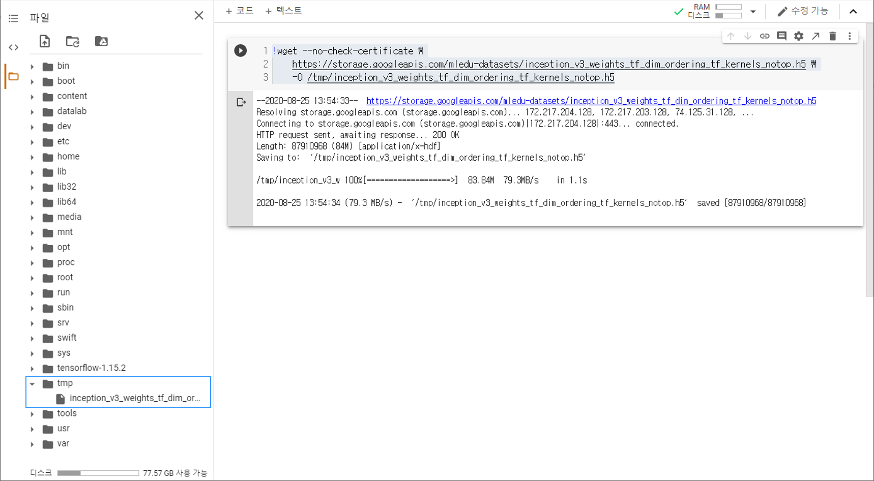
Google Colab환경에서 아래의 명령어를 실행하면, tmp 폴더에 미리 훈련된 가중치가 다운로드됩니다.
주소에 직접 접속해서 로컬 환경에 다운로드 받을 수도 있습니다.
!wget --no-check-certificate \
  https://storage.googleapis.com/mledu-datasets/inception_v3_weights_tf_dim_ordering_tf_kernels_notop.h5 \
  -O /tmp/inception_v3_weights_tf_dim_ordering_tf_kernels_notop.h5
--2020-08-25 13:54:33--  https://storage.googleapis.com/mledu-datasets/inception_v3_weights_tf_dim_ordering_tf_kernels_notop.h5
Resolving storage.googleapis.com (storage.googleapis.com)... 172.217.204.128, 172.217.203.128, 74.125.31.128, ...
Connecting to storage.googleapis.com (storage.googleapis.com)|172.217.204.128|:443... connected.
HTTP request sent, awaiting response... 200 OK
Length: 87910968 (84M) [application/x-hdf]
Saving to: ‘/tmp/inception_v3_weights_tf_dim_ordering_tf_kernels_notop.h5’

/tmp/inception_v3_w 100%[===================>]  83.84M  79.3MB/s    in 1.1s

2020-08-25 13:54:34 (79.3 MB/s) - ‘/tmp/inception_v3_weights_tf_dim_ordering_tf_kernels_notop.h5’ saved [87910968/87910968]
Google Colab 환경에서 아래와 같이 tmp 폴더에 파일이 생겼다면 전이 학습 (Transfer learning)을 활용할 준비가 되었습니다.
사전 훈련된 가중치 불러오기
import os
from tensorflow.keras import layers
from tensorflow.keras import Model
from tensorflow.keras.applications.inception_v3 import InceptionV3

local_weights_file = '/tmp/inception_v3_weights_tf_dim_ordering_tf_kernels_notop.h5'

pre_trained_model = InceptionV3(input_shape=(150, 150, 3),
                              include_top=False,
                              weights=None)

pre_trained_model.load_weights(local_weights_file)

for layer in pre_trained_model.layers:
  layer.trainable = False

pre_trained_model.summary()
Model: "inception_v3"
__________________________________________________________________________________________________
Layer (type)                    Output Shape         Param #     Connected to
==================================================================================================
input_1 (InputLayer)            [(None, 150, 150, 3) 0
__________________________________________________________________________________________________
conv2d (Conv2D)                 (None, 74, 74, 32)   864         input_1[0][0]
__________________________________________________________________________________________________
batch_normalization (BatchNorma (None, 74, 74, 32)   96          conv2d[0][0]
__________________________________________________________________________________________________
activation (Activation)         (None, 74, 74, 32)   0           batch_normalization[0][0]
__________________________________________________________________________________________________
conv2d_1 (Conv2D)               (None, 72, 72, 32)   9216        activation[0][0]
__________________________________________________________________________________________________
batch_normalization_1 (BatchNor (None, 72, 72, 32)   96          conv2d_1[0][0]
__________________________________________________________________________________________________
activation_1 (Activation)       (None, 72, 72, 32)   0           batch_normalization_1[0][0]
__________________________________________________________________________________________________
conv2d_2 (Conv2D)               (None, 72, 72, 64)   18432       activation_1[0][0]
__________________________________________________________________________________________________
batch_normalization_2 (BatchNor (None, 72, 72, 64)   192         conv2d_2[0][0]
__________________________________________________________________________________________________
activation_2 (Activation)       (None, 72, 72, 64)   0           batch_normalization_2[0][0]
__________________________________________________________________________________________________
max_pooling2d (MaxPooling2D)    (None, 35, 35, 64)   0           activation_2[0][0]
__________________________________________________________________________________________________
conv2d_3 (Conv2D)               (None, 35, 35, 80)   5120        max_pooling2d[0][0]
__________________________________________________________________________________________________
batch_normalization_3 (BatchNor (None, 35, 35, 80)   240         conv2d_3[0][0]
__________________________________________________________________________________________________
activation_3 (Activation)       (None, 35, 35, 80)   0           batch_normalization_3[0][0]
__________________________________________________________________________________________________
conv2d_4 (Conv2D)               (None, 33, 33, 192)  138240      activation_3[0][0]
__________________________________________________________________________________________________
batch_normalization_4 (BatchNor (None, 33, 33, 192)  576         conv2d_4[0][0]
__________________________________________________________________________________________________
activation_4 (Activation)       (None, 33, 33, 192)  0           batch_normalization_4[0][0]
__________________________________________________________________________________________________
max_pooling2d_1 (MaxPooling2D)  (None, 16, 16, 192)  0           activation_4[0][0]
__________________________________________________________________________________________________
conv2d_8 (Conv2D)               (None, 16, 16, 64)   12288       max_pooling2d_1[0][0]
__________________________________________________________________________________________________
batch_normalization_8 (BatchNor (None, 16, 16, 64)   192         conv2d_8[0][0]
__________________________________________________________________________________________________
activation_8 (Activation)       (None, 16, 16, 64)   0           batch_normalization_8[0][0]
__________________________________________________________________________________________________
conv2d_6 (Conv2D)               (None, 16, 16, 48)   9216        max_pooling2d_1[0][0]
__________________________________________________________________________________________________
conv2d_9 (Conv2D)               (None, 16, 16, 96)   55296       activation_8[0][0]
__________________________________________________________________________________________________
batch_normalization_6 (BatchNor (None, 16, 16, 48)   144         conv2d_6[0][0]
__________________________________________________________________________________________________
batch_normalization_9 (BatchNor (None, 16, 16, 96)   288         conv2d_9[0][0]
__________________________________________________________________________________________________

...
...

__________________________________________________________________________________________________
activation_87 (Activation)      (None, 3, 3, 384)    0           batch_normalization_87[0][0]
__________________________________________________________________________________________________
activation_88 (Activation)      (None, 3, 3, 384)    0           batch_normalization_88[0][0]
__________________________________________________________________________________________________
activation_91 (Activation)      (None, 3, 3, 384)    0           batch_normalization_91[0][0]
__________________________________________________________________________________________________
activation_92 (Activation)      (None, 3, 3, 384)    0           batch_normalization_92[0][0]
__________________________________________________________________________________________________
batch_normalization_93 (BatchNo (None, 3, 3, 192)    576         conv2d_93[0][0]
__________________________________________________________________________________________________
activation_85 (Activation)      (None, 3, 3, 320)    0           batch_normalization_85[0][0]
__________________________________________________________________________________________________
mixed9_1 (Concatenate)          (None, 3, 3, 768)    0           activation_87[0][0]
                                                               activation_88[0][0]
__________________________________________________________________________________________________
concatenate_1 (Concatenate)     (None, 3, 3, 768)    0           activation_91[0][0]
                                                               activation_92[0][0]
__________________________________________________________________________________________________
activation_93 (Activation)      (None, 3, 3, 192)    0           batch_normalization_93[0][0]
__________________________________________________________________________________________________
mixed10 (Concatenate)           (None, 3, 3, 2048)   0           activation_85[0][0]
                                                               mixed9_1[0][0]
                                                               concatenate_1[0][0]
                                                               activation_93[0][0]
==================================================================================================
Total params: 21,802,784
Trainable params: 0
Non-trainable params: 21,802,784
__________________________________________________________________________________________________
tensorflow.keras.applications 모듈은 사전 훈련된 가중치를 갖고 있는 다양한 신경망 구조를 포함합니다.
예제에서는 이 tensorflow.keras.applications 모듈의 inception_v3 모듈로부터 불러온 InceptionV3 함수를 사용해서 InceptionV3 모델을 구성합니다. InceptionV3 모델에 대해서는 링크1, 링크2를 참고하세요.
InceptionV3 모델은 상단 (출력층과 가까운 신경망의 끝부분)에 완전 연결된 뉴런층을 포함합니다.
include_top는 이러한 완전 연결된 뉴런층의 포함 여부를 설정합니다.
weights는 적용할 가중치를 지정합니다.
None: 임의로 초기화 (random initialization)된 가중치를 적용합니다.
imagenet: ImageNet에 대해 사전 훈련된 가중치를 적용합니다. (Default)
그 다음으로 load_weights() 메서드를 사용해서 미리 다운로드한 가중치를 InceptionV3 모델에 적용합니다.
layer.trainable는 뉴런층의 가중치의 훈련 가능 여부를 설정합니다.
summary() 메서드로 구성한 모델의 구조를 출력했습니다.
매우 많은 수의, 그리고 다양한 뉴런층이 포함되어 있음을 알 수 있습니다.
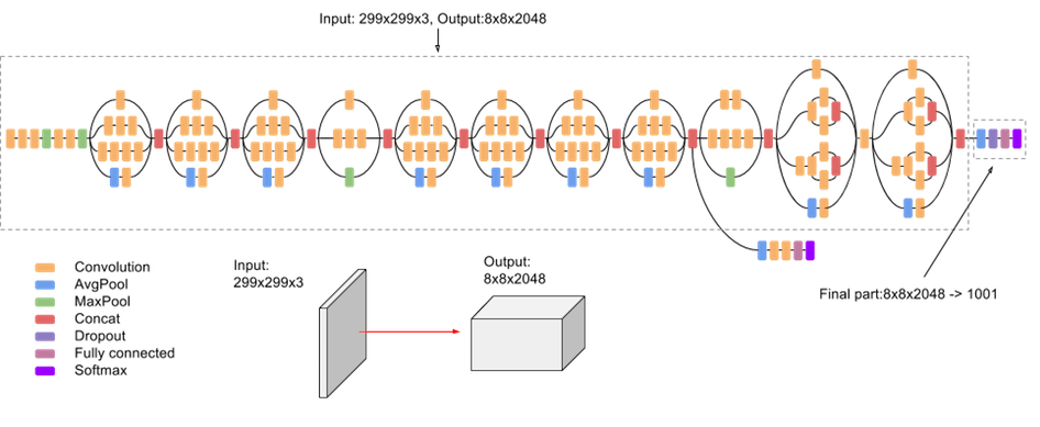
InceptionV3 모델의 구조를 그림으로 나타내면 아래와 같습니다.
마지막 층 출력 확인하기
last_layer = pre_trained_model.get_layer('mixed7')
print('last layer output shape: ', last_layer.output.shape)
last_output = last_layer.output
last layer output shape: (None, 7, 7, 768)
TensorFlow로 구성한 모델의 모든 뉴런층에는 이름이 있습니다.
앞에서 summary() 메서드로 모든 뉴런층의 이름을 출력했습니다.
‘mixed7’라는 이름을 갖는 층을 가져와서 사전 훈련된 신경망 모델의 마지막 층으로 지정했습니다.
모델 구성/컴파일하기
from tensorflow.keras.optimizers import RMSprop

x = layers.Flatten()(last_output)
x = layers.Dense(1024, activation='relu')(x)
x = layers.Dense(1, activation='sigmoid')(x)

model = Model(pre_trained_model.input, x)

model.compile(optimizer=RMSprop(lr=0.0001),
            loss='binary_crossentropy',
            metrics=['accuracy'])
Flatten()는 앞에서 지정한 InceptionV3 모델의 마지막 층의 출력을 1차원으로 변환합니다.
Dense()는 완전 연결된 뉴런층을 추가합니다.
두 개의 뉴런층을 추가하고 활성화 함수를 각각 ‘relu’와 ‘sigmoid’로 지정했습니다.
Model() 클래스에 InceptionV3 모델의 입력과 새롭게 구성한 뉴런층을 입력함으로써 새로운 모델을 만들었습니다.
compile()을 사용해서 구성한 모델을 컴파일합니다.
데이터셋 다운로드하기
사전 훈련된 가중치를 평가하기 위한 Kaggle Dogs Vs. Cats 데이터셋을 준비합니다.
Kaggle Dogs Vs. Cats 데이터셋에 대해서는 고양이와 개 이미지 분류하기 페이지를 참고하세요.
!wget --no-check-certificate \
        https://storage.googleapis.com/mledu-datasets/cats_and_dogs_filtered.zip \
       -O /tmp/cats_and_dogs_filtered.zip

import os
import zipfile

local_zip = '//tmp/cats_and_dogs_filtered.zip'

zip_ref = zipfile.ZipFile(local_zip, 'r')
zip_ref.extractall('/tmp')
zip_ref.close()
--2020-08-25 14:07:51--  https://storage.googleapis.com/mledu-datasets/cats_and_dogs_filtered.zip
Resolving storage.googleapis.com (storage.googleapis.com)... 173.194.216.128, 172.217.193.128, 172.217.204.128, ...
Connecting to storage.googleapis.com (storage.googleapis.com)|173.194.216.128|:443... connected.
HTTP request sent, awaiting response... 200 OK
Length: 68606236 (65M) [application/zip]
Saving to: ‘/tmp/cats_and_dogs_filtered.zip’

/tmp/cats_and_dogs_ 100%[===================>]  65.43M  83.2MB/s    in 0.8s

2020-08-25 14:07:52 (83.2 MB/s) - ‘/tmp/cats_and_dogs_filtered.zip’ saved [68606236/68606236]
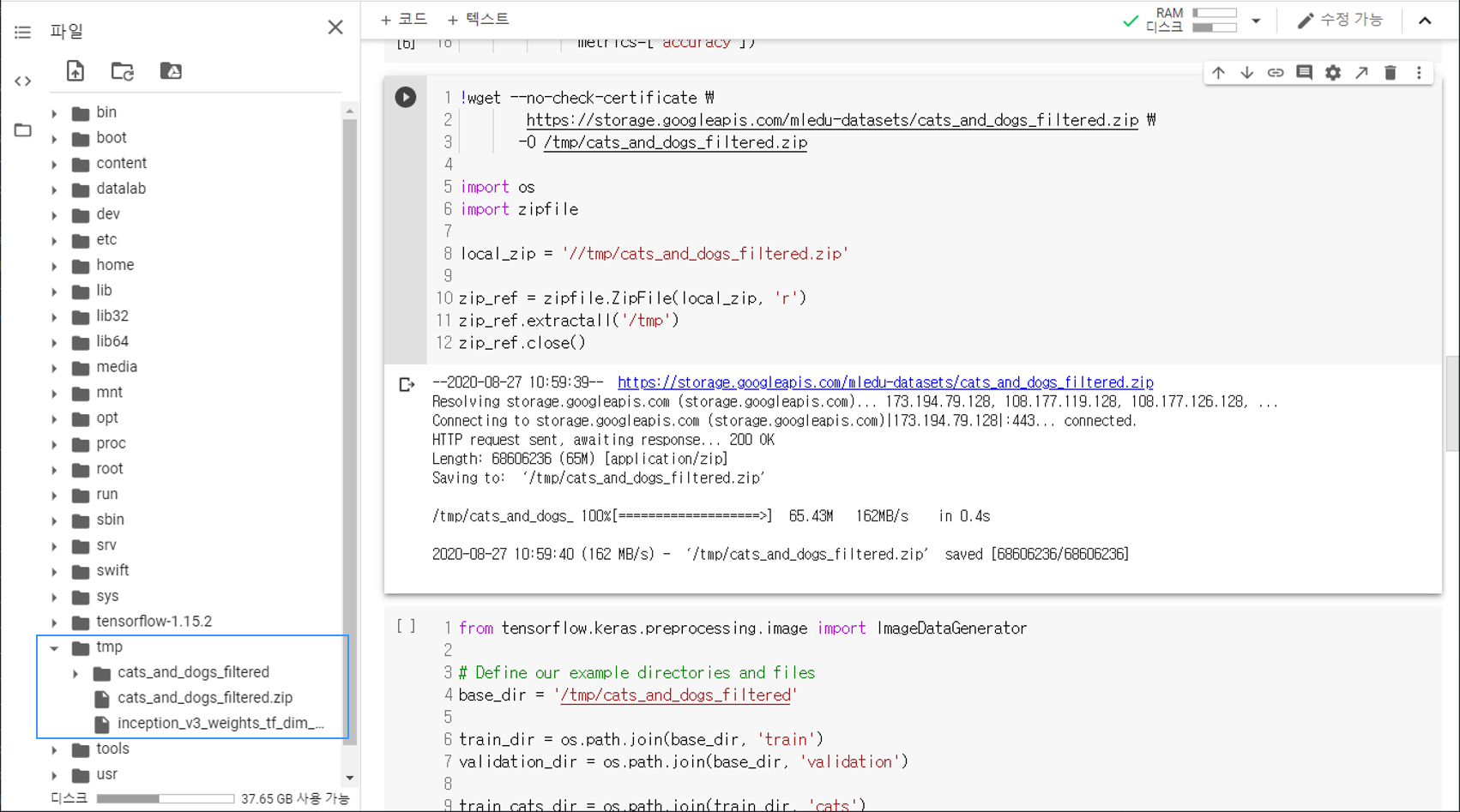
우선 Colab 코드셀에 위의 명령어를 입력해서 데이터셋을 다운로드합니다.
아래 그림과 같이 페이지 왼쪽의 목차 탭을 열어서 tmp 폴더에 cats_and_dogs_filtered.zip 파일이 다운로드되어 있는지 확인합니다.
cats_and_dogs_filtered.zip 파일이 준비되어 있다면 압축을 풀어줍니다.
데이터 어그멘테이션
from tensorflow.keras.preprocessing.image import ImageDataGenerator

# Define our example directories and files
base_dir = '/tmp/cats_and_dogs_filtered'

train_dir = os.path.join(base_dir, 'train')
validation_dir = os.path.join(base_dir, 'validation')

train_cats_dir = os.path.join(train_dir, 'cats')
train_dogs_dir = os.path.join(train_dir, 'dogs')
validation_cats_dir = os.path.join(validation_dir, 'cats')
validation_dogs_dir = os.path.join(validation_dir, 'dogs')

train_cat_fnames = os.listdir(train_cats_dir)
train_dog_fnames = os.listdir(train_dogs_dir)

# Add our data-augmentation parameters to ImageDataGenerator
train_datagen = ImageDataGenerator(rescale=1./255.,
                                 rotation_range=40,
                                 width_shift_range=0.2,
                                 height_shift_range=0.2,
                                 shear_range=0.2,
                                 zoom_range=0.2,
                                 horizontal_flip=True)

# Note that the validation data should not be augmented!
test_datagen = ImageDataGenerator(rescale=1./255.)

# Flow training images in batches of 20 using train_datagen generator
train_generator = train_datagen.flow_from_directory(train_dir,
                                                  batch_size=20,
                                                  class_mode='binary',
                                                  target_size=(150, 150))

# Flow validation images in batches of 20 using test_datagen generator
validation_generator = test_datagen.flow_from_directory(validation_dir,
                                                      batch_size=20,
                                                      class_mode='binary',
                                                      target_size=(150, 150))
Found 2000 images belonging to 2 classes.
Found 1000 images belonging to 2 classes.
이미지 어그멘테이션의 효과 페이지에서 다루었던대로 훈련 데이터에 대해 어그멘테이션을 활용합니다.
테스트 이미지에 대해서는 어그멘테이션을 수행하지 않고, 데이터 리스케일만 수행합니다.
모델 훈련하기
history = model.fit(
  train_generator,
  validation_data=validation_generator,
  steps_per_epoch=100,
  epochs=20,
  validation_steps=50,
  verbose=2
)
Epoch 1/20
100/100 - 24s - loss: 0.3288 - accuracy: 0.8760 - val_loss: 0.1874 - val_accuracy: 0.9310
Epoch 2/20
100/100 - 22s - loss: 0.2110 - accuracy: 0.9135 - val_loss: 0.0937 - val_accuracy: 0.9640
Epoch 3/20
100/100 - 23s - loss: 0.1942 - accuracy: 0.9245 - val_loss: 0.1157 - val_accuracy: 0.9580
Epoch 4/20
100/100 - 22s - loss: 0.1660 - accuracy: 0.9395 - val_loss: 0.1292 - val_accuracy: 0.9600
Epoch 5/20
100/100 - 23s - loss: 0.1758 - accuracy: 0.9340 - val_loss: 0.1013 - val_accuracy: 0.9570
Epoch 6/20
100/100 - 22s - loss: 0.1537 - accuracy: 0.9405 - val_loss: 0.0996 - val_accuracy: 0.9670
Epoch 7/20
100/100 - 23s - loss: 0.1583 - accuracy: 0.9440 - val_loss: 0.1099 - val_accuracy: 0.9620
Epoch 8/20
100/100 - 22s - loss: 0.1403 - accuracy: 0.9455 - val_loss: 0.0987 - val_accuracy: 0.9640
Epoch 9/20
100/100 - 23s - loss: 0.1583 - accuracy: 0.9450 - val_loss: 0.1143 - val_accuracy: 0.9640
Epoch 10/20
100/100 - 22s - loss: 0.1473 - accuracy: 0.9515 - val_loss: 0.0904 - val_accuracy: 0.9700
Epoch 11/20
100/100 - 22s - loss: 0.1444 - accuracy: 0.9485 - val_loss: 0.1099 - val_accuracy: 0.9640
Epoch 12/20
100/100 - 22s - loss: 0.1336 - accuracy: 0.9545 - val_loss: 0.1065 - val_accuracy: 0.9690
Epoch 13/20
100/100 - 22s - loss: 0.1250 - accuracy: 0.9570 - val_loss: 0.1657 - val_accuracy: 0.9550
Epoch 14/20
100/100 - 22s - loss: 0.1291 - accuracy: 0.9520 - val_loss: 0.1170 - val_accuracy: 0.9680
Epoch 15/20
100/100 - 22s - loss: 0.1268 - accuracy: 0.9585 - val_loss: 0.1100 - val_accuracy: 0.9630
Epoch 16/20
100/100 - 23s - loss: 0.1229 - accuracy: 0.9535 - val_loss: 0.1318 - val_accuracy: 0.9650
Epoch 17/20
100/100 - 22s - loss: 0.1062 - accuracy: 0.9545 - val_loss: 0.1317 - val_accuracy: 0.9700
Epoch 18/20
100/100 - 23s - loss: 0.1020 - accuracy: 0.9630 - val_loss: 0.1404 - val_accuracy: 0.9620
Epoch 19/20
100/100 - 22s - loss: 0.1184 - accuracy: 0.9580 - val_loss: 0.1313 - val_accuracy: 0.9670
Epoch 20/20
100/100 - 23s - loss: 0.1018 - accuracy: 0.9615 - val_loss: 0.1349 - val_accuracy: 0.9640
fit() 메서드를 사용해서, 20 에포크의 훈련을 수행합니다.
훈련 결과 확인하기
import matplotlib.pyplot as plt

acc = history.history['accuracy']
val_acc = history.history['val_accuracy']
loss = history.history['loss']
val_loss = history.history['val_loss']

epochs = range(len(acc))

plt.plot(epochs, acc, 'r', label='Training accuracy')
plt.plot(epochs, val_acc, 'b', label='Validation accuracy')
plt.title('Training and validation accuracy')
plt.legend(loc=0)
plt.figure()
plt.show()
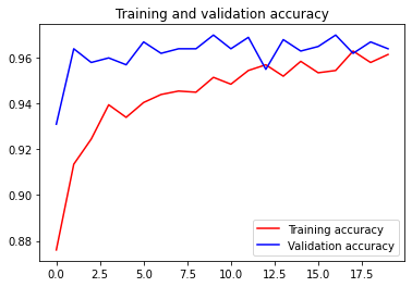
Matplotlib 라이브러리를 이용해서 훈련 과정을 시각화합니다.
20 에포크의 훈련 과정 동안 과적합 (Overfitting) 현상 없이 95% 이상의 훈련/테스트 정확도를 달성했습니다.