15. 다중 클래스 분류 문제

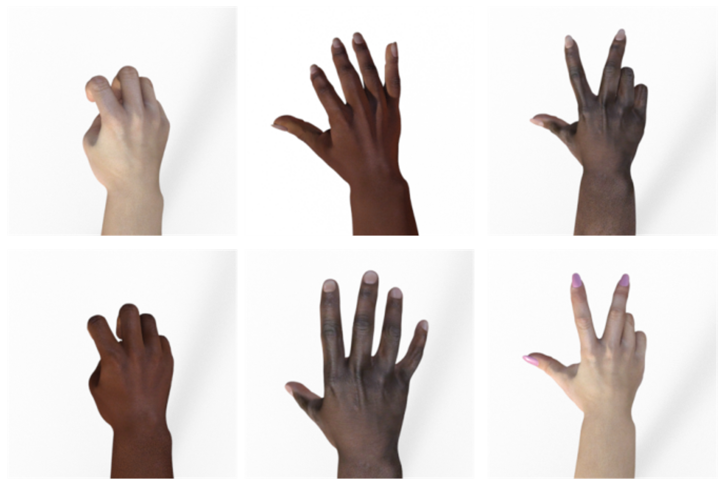
Rock Paper Scssors Datasets은 2,892개의 가위, 바위, 보 손동작 제스처 이미지를 포함하는 데이터셋입니다.

다양한 손동작, 인종, 나이, 성별의 가위, 바위, 보 이미지를 포함하며, 이미지에 해당하는 레이블을 포함합니다.

이미지들은 모두 CGI (Computer-Generated Imagery) 기술을 이용해서 생성되었습니다.

아래의 주소에서 훈련용 이미지와 테스트용 이미지를 다운로드받을 수 있습니다.

https://storage.googleapis.com/laurencemoroney-blog.appspot.com/rps.zip
https://storage.googleapis.com/laurencemoroney-blog.appspot.com/rps-test-set.zip

모든 이미지는 흰색 배경을 가지며, 24비트 색상의 300×300 픽셀로 이루어져 있습니다.

이 페이지에서는 세 개의 클래스를 갖는 데이터셋을 분류하는 방법에 대해서 소개합니다.

순서는 아래와 같습니다.

데이터셋 다운로드하기

Google Colab 환경에서 아래의 명령어를 실행하면, tmp 폴더에 Rock Paper Scssors Datasets이 다운로드됩니다.

주소에 직접 접속해서 로컬 환경에 다운로드 받을 수도 있습니다.

# 훈련용 이미지
!wget --no-check-certificate \
  https://storage.googleapis.com/laurencemoroney-blog.appspot.com/rps.zip \
  -O /tmp/rps.zip

--2020-09-01 12:56:07--  https://storage.googleapis.com/laurencemoroney-blog.appspot.com/rps.zip
Resolving storage.googleapis.com (storage.googleapis.com)... 173.194.69.128, 108.177.126.128, 108.177.127.128, ...
Connecting to storage.googleapis.com (storage.googleapis.com)|173.194.69.128|:443... connected.
HTTP request sent, awaiting response... 200 OK
Length: 200682221 (191M) [application/zip]
Saving to: ‘/tmp/rps.zip’

/tmp/rps.zip        100%[===================>] 191.38M  25.6MB/s    in 7.5s

2020-09-01 12:56:16 (25.6 MB/s) - ‘/tmp/rps.zip’ saved [200682221/200682221]

훈련용 이미지 데이터셋을 다운로드합니다.

# 테스트용 이미지
!wget --no-check-certificate \
  https://storage.googleapis.com/laurencemoroney-blog.appspot.com/rps-test-set.zip \
  -O /tmp/rps-test-set.zip

--2020-09-01 12:56:18--  https://storage.googleapis.com/laurencemoroney-blog.appspot.com/rps-test-set.zip
Resolving storage.googleapis.com (storage.googleapis.com)... 173.194.69.128, 108.177.126.128, 108.177.127.128, ...
Connecting to storage.googleapis.com (storage.googleapis.com)|173.194.69.128|:443... connected.
HTTP request sent, awaiting response... 200 OK
Length: 29516758 (28M) [application/zip]
Saving to: ‘/tmp/rps-test-set.zip’

/tmp/rps-test-set.z 100%[===================>]  28.15M  18.4MB/s    in 1.5s

2020-09-01 12:56:20 (18.4 MB/s) - ‘/tmp/rps-test-set.zip’ saved [29516758/29516758]

테스트용 이미지 데이터셋을 다운로드합니다.

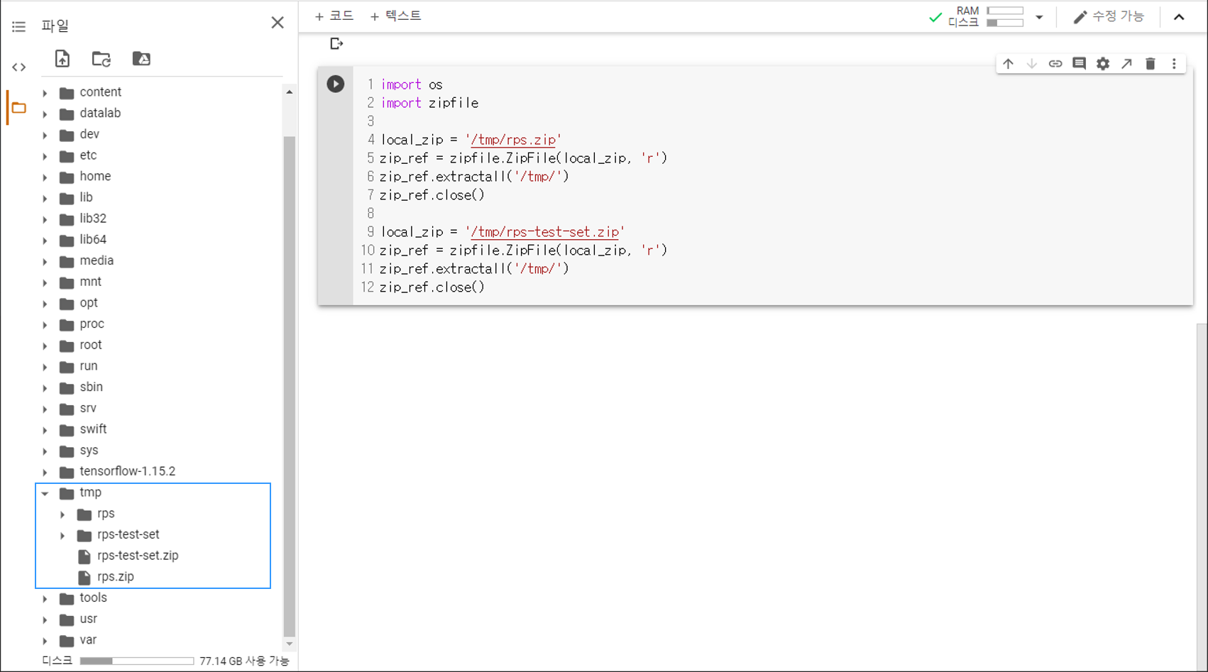
압출 풀기

import os
import zipfile

local_zip = '/tmp/rps.zip'
zip_ref = zipfile.ZipFile(local_zip, 'r')
zip_ref.extractall('/tmp/')
zip_ref.close()

local_zip = '/tmp/rps-test-set.zip'
zip_ref = zipfile.ZipFile(local_zip, 'r')
zip_ref.extractall('/tmp/')
zip_ref.close()

os 라이브러리를 통해 파일시스템에 접근할 수 있습니다.

zipfile 라이브러리의 ZipFile 클래스로 ZIP 파일을 연 후에

extractall() 메서드를 이용해서 tmp 폴더에 압축을 풉니다.

아래 그림과 같이 rps와 rps-test-set 폴더가 만들어졌다면 준비가 된 것입니다.

경로 지정하기

rock_dir = os.path.join('/tmp/rps/rock')
paper_dir = os.path.join('/tmp/rps/paper')
scissors_dir = os.path.join('/tmp/rps/scissors')

rock_files = os.listdir(rock_dir)
paper_files = os.listdir(paper_dir)
scissors_files = os.listdir(scissors_dir)

print('Total number of training rock images:', len(rock_files))
print('Total number of training paper images:', len(paper_files))
print('Total number of training scissors images:', len(scissors_files))

print(rock_files[:10])
print(paper_files[:10])
print(scissors_files[:10])

Total number of training rock images: 840
Total number of training paper images: 840
Total number of training scissors images: 840
['rock06ck02-084.png', 'rock07-k03-080.png', 'rock06ck02-023.png', 'rock07-k03-041.png', 'rock05ck01-103.png', 'rock02-046.png', 'rock06ck02-104.png', 'rock07-k03-088.png', 'rock02-031.png', 'rock03-116.png']
['paper03-095.png', 'paper07-064.png', 'paper04-028.png', 'paper05-081.png', 'paper04-016.png', 'paper03-020.png', 'paper03-031.png', 'paper03-067.png', 'paper06-017.png', 'paper04-101.png']
['testscissors03-047.png', 'testscissors02-040.png', 'scissors03-073.png', 'scissors04-081.png', 'scissors02-020.png', 'scissors04-117.png', 'testscissors03-069.png', 'scissors01-062.png', 'testscissors01-104.png', 'testscissors01-038.png']

훈련에 사용되는 가위, 바위, 보 (Scissors, Rock, Paper) 이미지의 경로를 각각 지정해줍니다.

각 클래스 별로 840개의 훈련용 이미지가 있음을 알 수 있습니다.

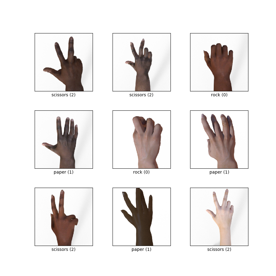
이미지 확인하기

%matplotlib inline

import matplotlib.pyplot as plt
import matplotlib.image as mpimg

pic_index = 2

next_rock = [os.path.join(rock_dir, fname) for fname in rock_files[pic_index-2:pic_index]]
next_paper = [os.path.join(paper_dir, fname) for fname in paper_files[pic_index-2:pic_index]]
next_scissors = [os.path.join(scissors_dir, fname) for fname in scissors_files[pic_index-2:pic_index]]

for i, img_path in enumerate(next_rock + next_paper + next_scissors):
  print(img_path)
  img = mpimg.imread(img_path)
  plt.imshow(img)
  plt.axis('Off')
  plt.show()

Matplotlib 라이브러리를 이용해서 각 클래스 별로 두 개의 이미지를 출력합니다.

아래와 같은 이미지들이 출력됩니다.

Neural Network 구성/훈련하기

import tensorflow as tf
import keras_preprocessing
from keras_preprocessing import image
from keras_preprocessing.image import ImageDataGenerator

TRAINING_DIR = "/tmp/rps/"
training_datagen = ImageDataGenerator(
    rescale = 1./255,
    rotation_range=40,
    width_shift_range=0.2,
    height_shift_range=0.2,
    shear_range=0.2,
    zoom_range=0.2,
    horizontal_flip=True,
    fill_mode='nearest')

VALIDATION_DIR = "/tmp/rps-test-set/"
validation_datagen = ImageDataGenerator(rescale = 1./255)

train_generator = training_datagen.flow_from_directory(
TRAINING_DIR,
target_size=(150,150),
class_mode='categorical',
batch_size=126
)

validation_generator = validation_datagen.flow_from_directory(
VALIDATION_DIR,
target_size=(150,150),
class_mode='categorical',
batch_size=126
)

model = tf.keras.models.Sequential([
  # Note the input shape is the desired size of the image 150x150 with 3 bytes color
  # This is the first convolution
  tf.keras.layers.Conv2D(64, (3,3), activation='relu', input_shape=(150, 150, 3)),
  tf.keras.layers.MaxPooling2D(2, 2),
  # The second convolution
  tf.keras.layers.Conv2D(64, (3,3), activation='relu'),
  tf.keras.layers.MaxPooling2D(2,2),
  # The third convolution
  tf.keras.layers.Conv2D(128, (3,3), activation='relu'),
  tf.keras.layers.MaxPooling2D(2,2),
  # The fourth convolution
  tf.keras.layers.Conv2D(128, (3,3), activation='relu'),
  tf.keras.layers.MaxPooling2D(2,2),
  # Flatten the results to feed into a DNN
  tf.keras.layers.Flatten(),
  tf.keras.layers.Dropout(0.5),
  # 512 neuron hidden layer
  tf.keras.layers.Dense(512, activation='relu'),
  tf.keras.layers.Dense(3, activation='softmax')
])


model.summary()

model.compile(loss = 'categorical_crossentropy', optimizer='rmsprop', metrics=['accuracy'])

history = model.fit(train_generator, epochs=25, steps_per_epoch=20, validation_data = validation_generator, verbose = 1, validation_steps=3)

model.save("rps.h5")

Found 2520 images belonging to 3 classes.
Found 372 images belonging to 3 classes.
Model: "sequential"
_________________________________________________________________
Layer (type)                 Output Shape              Param #
=================================================================
conv2d (Conv2D)              (None, 148, 148, 64)      1792
_________________________________________________________________
max_pooling2d (MaxPooling2D) (None, 74, 74, 64)        0
_________________________________________________________________
conv2d_1 (Conv2D)            (None, 72, 72, 64)        36928
_________________________________________________________________
max_pooling2d_1 (MaxPooling2 (None, 36, 36, 64)        0
_________________________________________________________________
conv2d_2 (Conv2D)            (None, 34, 34, 128)       73856
_________________________________________________________________
max_pooling2d_2 (MaxPooling2 (None, 17, 17, 128)       0
_________________________________________________________________
conv2d_3 (Conv2D)            (None, 15, 15, 128)       147584
_________________________________________________________________
max_pooling2d_3 (MaxPooling2 (None, 7, 7, 128)         0
_________________________________________________________________
flatten (Flatten)            (None, 6272)              0
_________________________________________________________________
dropout (Dropout)            (None, 6272)              0
_________________________________________________________________
dense (Dense)                (None, 512)               3211776
_________________________________________________________________
dense_1 (Dense)              (None, 3)                 1539
=================================================================
Total params: 3,473,475
Trainable params: 3,473,475
Non-trainable params: 0
_________________________________________________________________
Epoch 1/25
20/20 [==============================] - 18s 885ms/step - loss: 1.4556 - accuracy: 0.3496 - val_loss: 1.0823 - val_accuracy: 0.4651
Epoch 2/25
20/20 [==============================] - 18s 890ms/step - loss: 1.1098 - accuracy: 0.4103 - val_loss: 1.0265 - val_accuracy: 0.3952
Epoch 3/25
20/20 [==============================] - 18s 890ms/step - loss: 1.1098 - accuracy: 0.4675 - val_loss: 1.0414 - val_accuracy: 0.3333
Epoch 4/25
20/20 [==============================] - 18s 890ms/step - loss: 0.9462 - accuracy: 0.5381 - val_loss: 0.6964 - val_accuracy: 0.6452
Epoch 5/25
20/20 [==============================] - 18s 888ms/step - loss: 0.8694 - accuracy: 0.6702 - val_loss: 0.8906 - val_accuracy: 0.5134
Epoch 6/25
20/20 [==============================] - 18s 886ms/step - loss: 0.6766 - accuracy: 0.6972 - val_loss: 0.4299 - val_accuracy: 0.7204
Epoch 7/25
20/20 [==============================] - 18s 894ms/step - loss: 0.5805 - accuracy: 0.7429 - val_loss: 0.1932 - val_accuracy: 1.0000
Epoch 8/25
20/20 [==============================] - 18s 889ms/step - loss: 0.4697 - accuracy: 0.8147 - val_loss: 0.0851 - val_accuracy: 1.0000
Epoch 9/25
20/20 [==============================] - 18s 888ms/step - loss: 0.3671 - accuracy: 0.8460 - val_loss: 0.4870 - val_accuracy: 0.6935
Epoch 10/25
20/20 [==============================] - 18s 889ms/step - loss: 0.3455 - accuracy: 0.8631 - val_loss: 0.0311 - val_accuracy: 1.0000
Epoch 11/25
20/20 [==============================] - 18s 892ms/step - loss: 0.3319 - accuracy: 0.8813 - val_loss: 0.1506 - val_accuracy: 0.9274
Epoch 12/25
20/20 [==============================] - 18s 889ms/step - loss: 0.2329 - accuracy: 0.9115 - val_loss: 0.0231 - val_accuracy: 1.0000
Epoch 13/25
20/20 [==============================] - 18s 888ms/step - loss: 0.2997 - accuracy: 0.9083 - val_loss: 0.0118 - val_accuracy: 1.0000
Epoch 14/25
20/20 [==============================] - 18s 888ms/step - loss: 0.1999 - accuracy: 0.9258 - val_loss: 0.0142 - val_accuracy: 1.0000
Epoch 15/25
20/20 [==============================] - 18s 895ms/step - loss: 0.1527 - accuracy: 0.9504 - val_loss: 0.0109 - val_accuracy: 1.0000
Epoch 16/25
20/20 [==============================] - 18s 902ms/step - loss: 0.4454 - accuracy: 0.8722 - val_loss: 0.0479 - val_accuracy: 0.9839
Epoch 17/25
20/20 [==============================] - 18s 890ms/step - loss: 0.1210 - accuracy: 0.9595 - val_loss: 0.0065 - val_accuracy: 1.0000
Epoch 18/25
20/20 [==============================] - 18s 886ms/step - loss: 0.2171 - accuracy: 0.9190 - val_loss: 0.0083 - val_accuracy: 1.0000
Epoch 19/25
20/20 [==============================] - 18s 885ms/step - loss: 0.1154 - accuracy: 0.9552 - val_loss: 0.0375 - val_accuracy: 0.9892
Epoch 20/25
20/20 [==============================] - 18s 891ms/step - loss: 0.1721 - accuracy: 0.9377 - val_loss: 0.1403 - val_accuracy: 0.9301
Epoch 21/25
20/20 [==============================] - 18s 886ms/step - loss: 0.1019 - accuracy: 0.9667 - val_loss: 0.0147 - val_accuracy: 1.0000
Epoch 22/25
20/20 [==============================] - 18s 886ms/step - loss: 0.2504 - accuracy: 0.9278 - val_loss: 0.0369 - val_accuracy: 0.9892
Epoch 23/25
20/20 [==============================] - 18s 887ms/step - loss: 0.0775 - accuracy: 0.9734 - val_loss: 0.0141 - val_accuracy: 1.0000
Epoch 24/25
20/20 [==============================] - 18s 894ms/step - loss: 0.0672 - accuracy: 0.9770 - val_loss: 0.0072 - val_accuracy: 1.0000
Epoch 25/25
20/20 [==============================] - 18s 888ms/step - loss: 0.2173 - accuracy: 0.9278 - val_loss: 0.0118 - val_accuracy: 1.0000

25회 에포크의 훈련을 진행합니다.

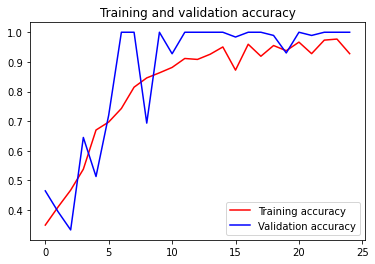
훈련 결과 확인하기

import matplotlib.pyplot as plt
acc = history.history['accuracy']
val_acc = history.history['val_accuracy']
loss = history.history['loss']
val_loss = history.history['val_loss']

epochs = range(len(acc))

plt.plot(epochs, acc, 'r', label='Training accuracy')
plt.plot(epochs, val_acc, 'b', label='Validation accuracy')
plt.title('Training and validation accuracy')
plt.legend(loc=0)
plt.figure()
plt.show()

훈련용, 테스트용 데이터에 대한 정확도를 나타내면 아래와 같습니다.

이전글/다음글

이전글 : 14. 전이 학습 활용하기

다음글 : 16. 시냅스 가중치 얻기

공유하기