시계열 데이터 기초

이 페이지에서는 시계열 데이터 (Time Series Data)의 기본적인 특징에 대해 소개합니다.

그리고 NumPy를 이용해서 시계열 데이터를 만들고, Matplotlib를 이용해서 시각화합니다.

시계열 데이터 시각화 함수

예제

import numpy as np
import matplotlib.pyplot as plt
import tensorflow as tf
from tensorflow import keras

plt.style.use('default')
plt.rcParams['figure.figsize'] = (6, 3)
plt.rcParams['font.size'] = 12

def plot_series(time, series, format="-", start=0, end=None, label=None):
    plt.plot(time[start:end], series[start:end], format, label=label)
    plt.xlabel("Time")
    plt.ylabel("Value")
    if label:
        plt.legend(fontsize=14)
    plt.grid(True)

plot_series() 함수는 임의의 시간 값 (time), 시계열 데이터 (series)를 입력받아 Matplotlib 그래프로 나타내는 함수입니다.

X, Y축 레이블을 각각 ‘Time’, ‘Value’로 지정하고, 데이터 영역에 그리드를 표시했습니다.

Matplotlib 축 레이블 설정하기, 그리드 설정하기 페이지를 참고하세요.

아래의 예제에서 계속해서 이 함수를 사용합니다.

경향성을 갖는 시계열 데이터

예제

def trend(time, slope=0):
    return slope * time

time = np.arange(4 * 365 + 1)
series = trend(time, slope=0.1)

plot_series(time, series)
plt.show()

trend() 함수는 경향성을 갖는 시계열 데이터를 반환합니다.

slope 값에 따라서 시간에 따라 양의 경향성, 음의 경향성을 가질 수 있습니다.

예제에서는 길이 4 * 365 + 1의 시간 동안 시간에 따라 0.1의 기울기를 갖는 시계열 데이터를 만들었습니다.

아래와 같은 데이터가 만들어집니다.

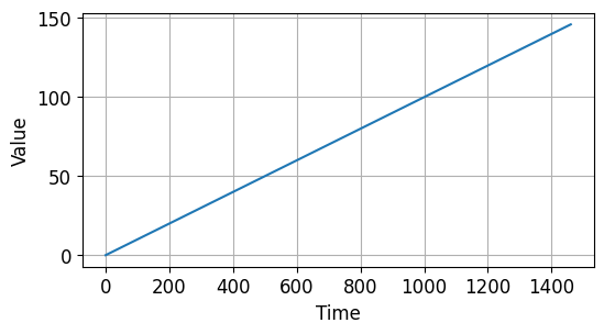
시계열 데이터 기초 - 경향성을 갖는 시계열 데이터

계절성을 갖는 시계열 데이터

예제1

def seasonal_pattern(season_time):
    return np.where(season_time < 0.6,
                    np.cos(season_time * 2 * np.pi),
                    1 / np.exp(3 * season_time))

def seasonality(time, period, amplitude=1, phase=0):
    season_time = ((time + phase) % period) / period
    return amplitude * seasonal_pattern(season_time)

amplitude = 40
series = seasonality(time, period=365, amplitude=amplitude)

plot_series(time, series)
plt.show()

seasonal_pattern() 함수는 입력 season_time에 대해서 0.6보다 작은 경우에는 np.cos(season_time * 2 * np.pi) 값을,

그렇지 않은 경우에는 1 / np.exp(3 * season_time)을 반환합니다.

NumPy 다양한 함수들 - numpy.where 페이지를 참고하세요.

seasonality() 함수는 주어진 주기 period에 대해 특정 값을 반복하는 시계열 데이터를 반환하는 함수입니다.

아래와 같은 시계열 데이터가 만들어졌습니다.

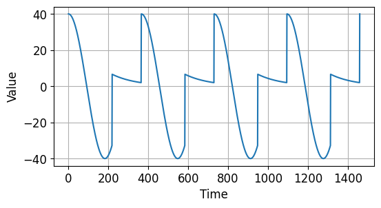
시계열 데이터 기초 - 계절성을 갖는 시계열 데이터

예제2

baseline = 10
slope = 0.05
series = baseline + trend(time, slope) + seasonality(time, period=365, amplitude=amplitude)

plot_series(time, series)
plt.show()

trend(), seasonality() 함수를 사용해서 경향성 (Trend)과 계절성 (Seasonality)을 모두 갖는 시계열 데이터를 만들었습니다.

아래와 같은 시계열 데이터가 만들어졌습니다.

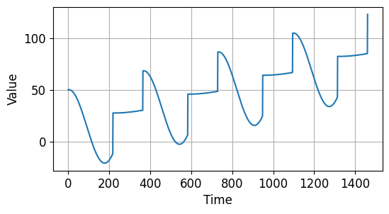
시계열 데이터 기초 - 경향성/계절성을 갖는 시계열 데이터

노이즈를 갖는 시계열 데이터

예제1

def white_noise(time, noise_level=1, seed=None):
    rnd = np.random.RandomState(seed)
    return rnd.rand(len(time)) * noise_level

noise_level = 5
noise = white_noise(time, noise_level, seed=42)

plot_series(time, noise)
plt.show()

white_noise() 함수는 0에서 noise_level 값 사이의 임의의 실수를 갖는 시계열 데이터를 반환합니다.

아래와 같은 시계열 데이터가 만들어졌습니다.

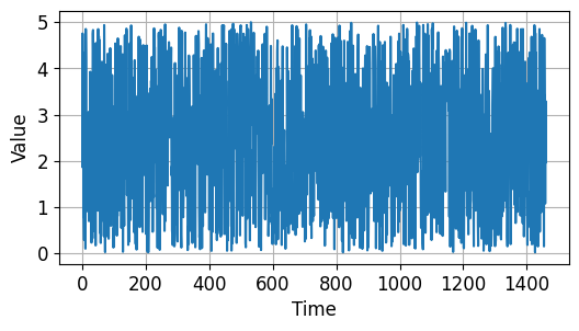
시계열 데이터 기초 - 노이즈를 갖는 시계열 데이터

예제2

baseline = 10
slope = 0.05
noise_level = 5
series = baseline + trend(time, slope) + seasonality(time, period=365, amplitude=amplitude) \
        + white_noise(time, noise_level, seed=42)

plot_series(time, series)
plt.show()

이번에는 경향성 (Trend), 계절성 (Seasonality)과 노이즈 (Noise)를 모두 갖는 시계열 데이터를 만들었습니다.

아래와 같습니다.

시계열 데이터 기초 - 경향성, 계절성, 노이즈를 갖는 시계열 데이터

자기상관성을 갖는 시계열 데이터

예제1

split_time = 1000
time_train, x_train = time[:split_time], series[:split_time]
time_valid, x_valid = time[split_time:], series[split_time:]

def autocorrelation(time, amplitude, seed=None):
    rnd = np.random.RandomState(seed)
    pi = 0.8
    ar =  rnd.randn(len(time) + 1)
    for step in range(1, len(time) + 1):
        ar[step] += pi * ar[step - 1]       ## 이전의 값의 0.8배를 더하기
    return ar[1:] * amplitude

series = autocorrelation(time, 10, seed=42)
plot_series(time[:200], series[:200])
plt.show()

autocorrelation() 함수는 자기상관성 (Autocorrelation)을 갖는 시계열 데이터를 반환합니다.

ar은 정규분포를 갖는 임의의 데이터입니다.

이전 시간 스텝 값의 0.8배를 더해주고, 크기 amplitude를 곱한 시계열 데이터를 반환합니다.

시계열 데이터 기초 - 자기상관성을 갖는 시계열 데이터

예제2

series = autocorrelation(time, 10, seed=42) + trend(time, 2)
plot_series(time[:200], series[:200])
plt.show()

자기상관성 (Autocorrelation)과 경향성 (Trend)을 갖는 시계열 데이터를 만들었습니다.

결과는 아래와 같습니다.

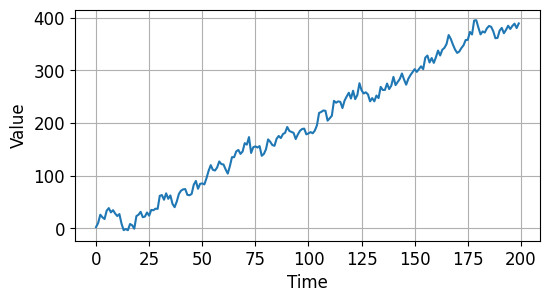
시계열 데이터 기초 - 자기상관성과 경향성을 갖는 시계열 데이터

예제3

series = autocorrelation(time, 10, seed=42) + seasonality(time, period=50, amplitude=150) + trend(time, 2)
plot_series(time[:200], series[:200])
plt.show()

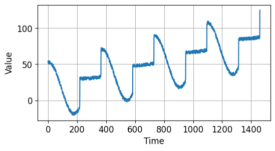
이번에는 자기상관성 (Autocorrelation), 경향성 (Trend)과 함께 계절성 (Seasonality)을 갖는 시계열 데이터를 만들었습니다.

아래와 같습니다.

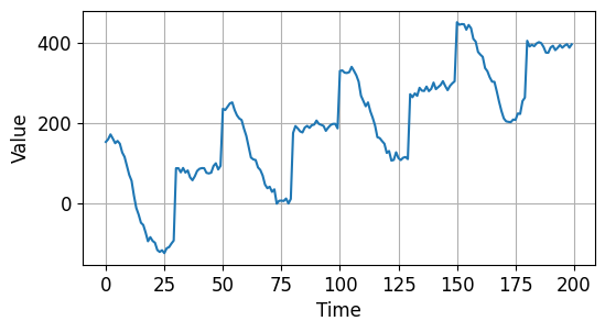
시계열 데이터 기초 - 자기상관성, 경향성, 계절성을 갖는 시계열 데이터

예제4

series = autocorrelation(time, 10, seed=42) + seasonality(time, period=50, amplitude=150) + trend(time, 2)
series2 = autocorrelation(time, 5, seed=42) + seasonality(time, period=50, amplitude=2) + trend(time, -1) + 550
series[200:] = series2[200:]        # 자기상관 amp 10->5, 계절성 amp 150->2, 경향성 slope 2->-1 + 550
series += white_noise(time, 30)
plot_series(time[:300], series[:300])
plt.show()

이번에는 특정 시점 이후로 다른 특성을 갖는 시계열 데이터를 만들어보겠습니다.

2/3 지점 이후로 크기 (amplitude)와 주기 (period), 경향성 (slope)이 모두 달라진 특성을 갖는 시계열 데이터입니다.

또한 전체 구간에서 노이즈 (Noise)를 갖습니다.

결과는 아래와 같습니다.

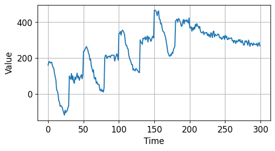
시계열 데이터 기초 - 특정 시점 이후 변화 추세를 갖는 시계열 데이터

이전글/다음글

이전글 : 21. 시계열 데이터 예측하기

다음글 : 시계열 데이터 예측하기

공유하기