순환 신경망 사용하기

순환 신경망 (Recurrent Neural Network)은 시계열 데이터에 적합한 형태의 신경망입니다.

순환 신경망은 입력된 데이터들에 대한 정보를 유지하면서 시계열 데이터를 처리합니다.

아래의 코드를 앞에서 작성한 코드에 이어서 작성합니다.

shuffle, batch, cache

tf.data를 이용해서 데이터셋을 shuffle, batch, cache하는 작업을 수행합니다.

train_univariate = tf.data.Dataset.from_tensor_slices((x_train_uni, y_train_uni))
train_univariate = train_univariate.cache().shuffle(BUFFER_SIZE).batch(BATCH_SIZE).repeat()

val_univariate = tf.data.Dataset.from_tensor_slices((x_val_uni, y_val_uni))
val_univariate = val_univariate.batch(BATCH_SIZE).repeat()

tf.data.Dataset의 from_tensor_slices()는 주어진 텐서들 ((x_train_uni, y_train_uni))을 첫번째 차원을 따라 슬라이스합니다.

모든 입력 텐서는 첫번째 차원과 같은 크기를 가져야합니다.

from_tensor_slices()를 사용하는 간단한 예를 보면,

x_train_uni = [[[1], [2]], [[3], [4]], [[5], [6]]]
y_train_uni = [0.1, 0.2, 0.3]

train_univariate = tf.data.Dataset.from_tensor_slices((x_train_uni, y_train_uni))
print(train_univariate)
print(list(train_univariate))

<TensorSliceDataset shapes: ((2, 1), ()), types: (tf.int32, tf.float32)>
[(<tf.Tensor: id=8, shape=(2, 1), dtype=int32, numpy=
array([[1],
       [2]], dtype=int32)>, <tf.Tensor: id=9, shape=(), dtype=float32, numpy=0.1>), (<tf.Tensor: id=10, shape=(2, 1), dtype=int32, numpy=
array([[3],
       [4]], dtype=int32)>, <tf.Tensor: id=11, shape=(), dtype=float32, numpy=0.2>), (<tf.Tensor: id=12, shape=(2, 1), dtype=int32, numpy=
array([[5],
       [6]], dtype=int32)>, <tf.Tensor: id=13, shape=(), dtype=float32, numpy=0.3>)]

x_train_uni = [[[1], [2]], [[3], [4]], [[5], [6]]]와 y_train_uni = [0.1, 0.2, 0.3]에 대해,

각각의 텐서를 슬라이스해서 새로운 데이터셋이 만들어졌습니다.

cache()는 데이터셋을 캐시, 즉 메모리 또는 파일에 보관합니다. 따라서 두번째 이터레이션부터는 캐시된 데이터를 사용합니다.

shuffle()는 데이터셋을 임의로 섞어줍니다. BUFFER_SIZE개로 이루어진 버퍼로부터 임의로 샘플을 뽑고, 뽑은 샘플은 다른 샘플로 대체합니다. 완벽한 셔플을 위해서 전체 데이터셋의 크기에 비해 크거나 같은 버퍼 크기가 요구됩니다.

batch()는 데이터셋의 항목들을 하나의 배치로 묶어줍니다.

아래의 그림은 배치 작업이 이루어진 후의 데이터가 어떻게 구성되는지 나타냅니다.

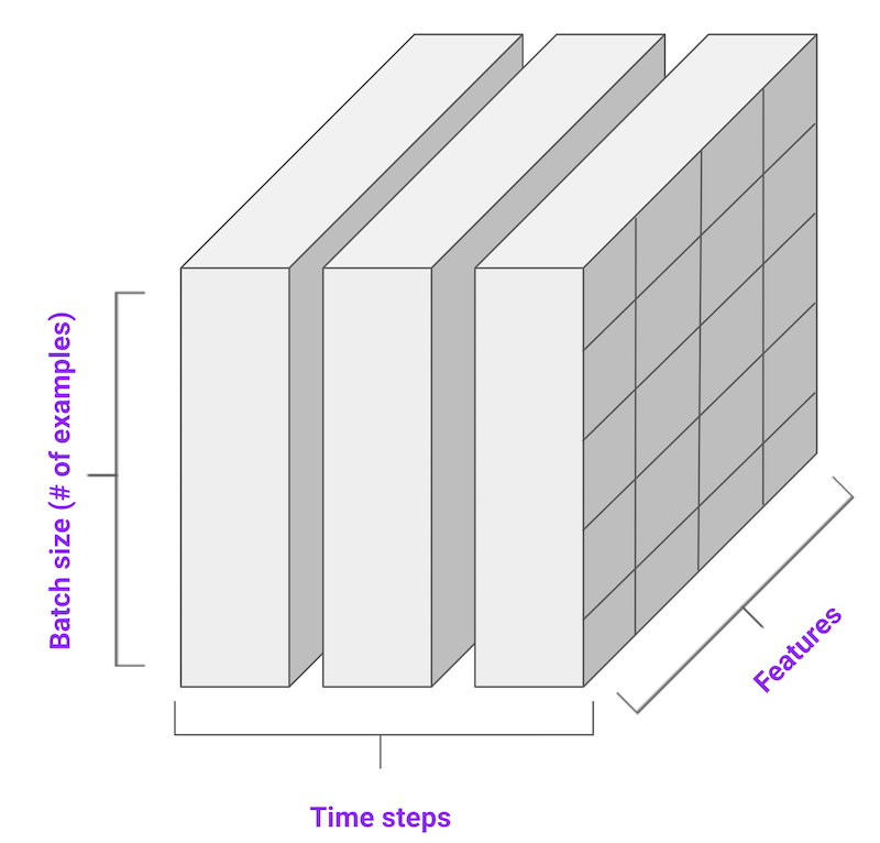
(그림: tensorflow.org)

LSTM (Long Short Term Memory)

LSTM은 순환 신경망 (RNN)의 특수한 형태입니다. 아래의 코드를 통해 간단한 LSTM 모델을 구성합니다.

simple_lstm_model = tf.keras.models.Sequential([
    tf.keras.layers.LSTM(8, input_shape=x_train_uni.shape[-2:]),
    tf.keras.layers.Dense(1)
])

simple_lstm_model.compile(optimizer='adam', loss='mae')

그리고 모델을 훈련합니다.

EVALUATION_INTERVAL = 200
EPOCHS = 10

simple_lstm_model.fit(train_univariate, epochs=EPOCHS,
                      steps_per_epoch=EVALUATION_INTERVAL,
                      validation_data=val_univariate, validation_steps=50)

Epoch 1/10
200/200 [==============================] - 5s 23ms/step - loss: 0.4075 - val_loss: 0.1351
Epoch 2/10
200/200 [==============================] - 3s 16ms/step - loss: 0.1118 - val_loss: 0.0359
Epoch 3/10
200/200 [==============================] - 3s 14ms/step - loss: 0.0489 - val_loss: 0.0290
Epoch 4/10
200/200 [==============================] - 3s 14ms/step - loss: 0.0443 - val_loss: 0.0258
Epoch 5/10
200/200 [==============================] - 3s 14ms/step - loss: 0.0299 - val_loss: 0.0235
Epoch 6/10
200/200 [==============================] - 3s 14ms/step - loss: 0.0317 - val_loss: 0.0224
Epoch 7/10
200/200 [==============================] - 3s 13ms/step - loss: 0.0286 - val_loss: 0.0206
Epoch 8/10
200/200 [==============================] - 3s 13ms/step - loss: 0.0263 - val_loss: 0.0200
Epoch 9/10
200/200 [==============================] - 3s 13ms/step - loss: 0.0254 - val_loss: 0.0182
Epoch 10/10
200/200 [==============================] - 3s 13ms/step - loss: 0.0228 - val_loss: 0.0173

훈련이 이루어졌습니다.

이제 이 간단한 LSTM 모델을 이용한 예측을 확인합니다.

for x, y in val_univariate.take(3):
    plot = show_plot([x[0].numpy(), y[0].numpy(),
                      simple_lstm_model.predict(x)[0]], 0, 'Simple LSTM model')
    plot.show()

결과는 아래와 같습니다.

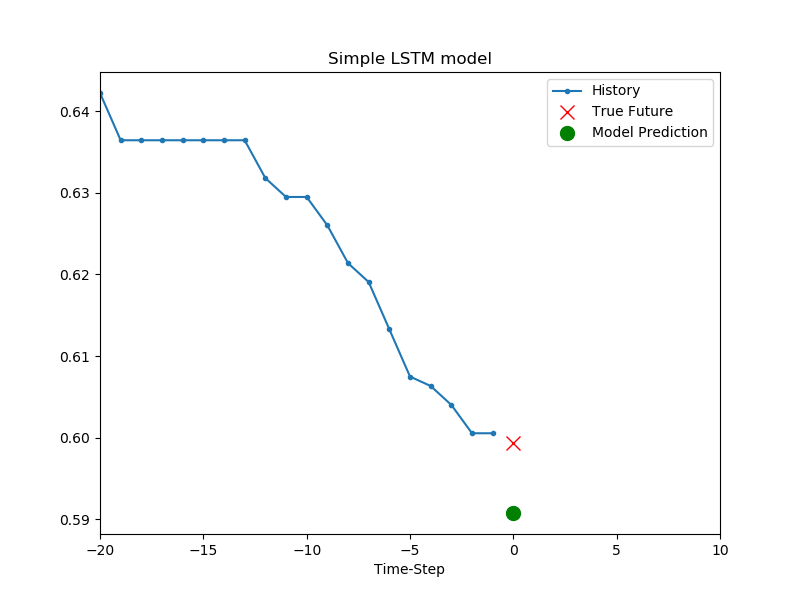
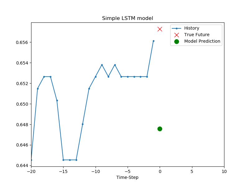
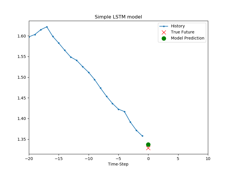
간단한 LSTM을 모델을 이용한 예측.

baseline() 함수가 했던 과거 20개의 온도 데이터의 평균을 사용한 예측보다 개선된 결과를 확인할 수 있습니다.

이제 온도 데이터만이 아닌 다변량 시계열 (multivariate time series) 데이터를 다뤄 보겠습니다.

지금까지 작성한 코드는 아래와 같습니다.

import tensorflow as tf
import matplotlib as mpl
import matplotlib.pyplot as plt
import numpy as np
import os
import pandas as pd

mpl.rcParams['figure.figsize'] = (8, 6)
mpl.rcParams['axes.grid'] = False

zip_path = tf.keras.utils.get_file(
    origin='https://storage.googleapis.com/tensorflow/tf-keras-datasets/jena_climate_2009_2016.csv.zip',
    fname='jena_climate_2009_2016.csv.zip',
    extract=True)
csv_path, _ = os.path.splitext(zip_path)

df = pd.read_csv(csv_path)
# print(df.head())
# print(df.columns)


def univariate_data(dataset, start_index, end_index, history_size, target_size):
    data = []
    labels = []

    start_index = start_index + history_size
    if end_index is None:
        end_index = len(dataset) - target_size

    for i in range(start_index, end_index):
        indices = range(i - history_size, i)
        # Reshape data from (history_size,) to (history_size, 1)
        data.append(np.reshape(dataset[indices], (history_size, 1)))
        labels.append(dataset[i+target_size])
    return np.array(data), np.array(labels)


TRAIN_SPLIT = 300000
tf.random.set_seed(13)

uni_data = df['T (degC)']
uni_data.index = df['Date Time']
# print(uni_data.head())

# uni_data.plot(subplots=True)
# plt.show()

uni_data = uni_data.values
uni_train_mean = uni_data[:TRAIN_SPLIT].mean()
uni_train_std = uni_data[:TRAIN_SPLIT].std()
uni_data = (uni_data - uni_train_mean) / uni_train_std  # Standardization

# print(uni_data)

univariate_past_history = 20
univariate_future_target = 0

x_train_uni, y_train_uni = univariate_data(uni_data, 0, TRAIN_SPLIT,
                                           univariate_past_history,
                                           univariate_future_target)
x_val_uni, y_val_uni = univariate_data(uni_data, TRAIN_SPLIT, None,
                                       univariate_past_history,
                                       univariate_future_target)

# print('Single window of past history')
# print(x_train_uni[0])
# print('\n Target temperature to predict')
# print(y_train_uni[0])


def create_time_steps(length):
    return list(range(-length, 0))


def show_plot(plot_data, delta, title):
    labels = ['History', 'True Future', 'Model Prediction']
    marker = ['.-', 'rx', 'go']
    time_steps = create_time_steps(plot_data[0].shape[0])
    if delta:
        future = delta
    else:
        future = 0

    plt.title(title)
    for i, x in enumerate(plot_data):
        if i:
            plt.plot(future, plot_data[i], marker[i], markersize=10, label=labels[i])
        else:
            plt.plot(time_steps, plot_data[i].flatten(), marker[i], label=labels[i])
    plt.legend()
    plt.axis('auto')
    plt.xlim([time_steps[0], (future+5)*2])
    plt.xlabel('Time-Step')
    return plt


# show_plot([x_train_uni[0], y_train_uni[0]], 0, 'Sample Example').show()


def baseline(history):
    return np.mean(history)


# show_plot([x_train_uni[0], y_train_uni[0], baseline(x_train_uni[0])], 0, 'Sample Example').show()

BATCH_SIZE = 256
BUFFER_SIZE = 10000

train_univariate = tf.data.Dataset.from_tensor_slices((x_train_uni, y_train_uni))
train_univariate = train_univariate.cache().shuffle(BUFFER_SIZE).batch(BATCH_SIZE).repeat()

val_univariate = tf.data.Dataset.from_tensor_slices((x_val_uni, y_val_uni))
val_univariate = val_univariate.batch(BATCH_SIZE).repeat()

simple_lstm_model = tf.keras.models.Sequential([
    tf.keras.layers.LSTM(8, input_shape=x_train_uni.shape[-2:]),
    tf.keras.layers.Dense(1)
])

simple_lstm_model.compile(optimizer='adam', loss='mae')

EVALUATION_INTERVAL = 200
EPOCHS = 10

simple_lstm_model.fit(train_univariate, epochs=EPOCHS,
                      steps_per_epoch=EVALUATION_INTERVAL,
                      validation_data=val_univariate, validation_steps=50)

for x, y in val_univariate.take(3):
    plot = show_plot([x[0].numpy(), y[0].numpy(),
                      simple_lstm_model.predict(x)[0]], 0, 'Simple LSTM model')
    plot.show()

이전글/다음글

이전글 : 단변량 시계열 데이터 예측하기

다음글 : 다변량 시계열 데이터 예측하기

공유하기